Description
Velocity model is the key component in the seismic imaging. Be it a time imaging or depth imaging. To achieve the best velocity model, geophysical community around the world uses various methods like tomography (grid tomography, stereo tomography etc), FWI (Full Wave Inversion) etc.
To start with, we need a good initial velocity model. From the time imaging, we take Vrms velocity model and convert that into Vinterval depth velocity model. To perform this within g-Platform, the user should use either Grid tomography 2D/3D module or Dix TV module to generate the Vinterval depth velocity model from the initial Vrms velocity model.
The Grid Tomography 2D / 3D module converts an input RMS (root-mean-square) velocity model into an interval depth velocity model using a CRS (Common Reflection Surface) based tomographic inversion. The algorithm distributes a regular grid of knot points throughout the subsurface volume and performs iterative least-squares inversion to solve for the interval velocity at each grid node. Multiple global iterations progressively refine the grid resolution, starting from a coarse grid and decreasing cell size by the specified resolution factor, ensuring that large-scale velocity trends are established first before fine-scale detail is resolved.
The module supports both 2D and 3D survey geometries. In 2D mode, the inversion operates in the X-Z plane only. In 3D mode, the full X-Y-Z volume is inverted simultaneously. The result is a smooth, geologically consistent interval velocity model suitable for use as input to depth migration workflows or further velocity model building iterations.
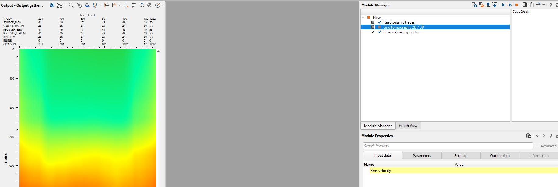
In the above image, we read the initial Vrms velocity model by using "Read seismic traces" module. We connect the initial Vrms velocity model to Grid tomography 2D/3D module. As per our data we need to set up our parameters. In this example we are showing the parameters for a 2D case.
Few parameters are worth mentioning here. Unlike the time imaging where the migration runs from the topography, depth imaging runs from the datum. So the user should provide the datum value in the respective field.
Input data
Rms velocity
Connect the input RMS velocity model here. This is typically a velocity gather where each trace represents the RMS velocity function at a surface location, sampled in two-way travel time. The module reads the spatial coordinates and velocity values from this gather to drive the tomographic inversion. The data must carry correct bin coordinates (X and Y picket values) for the spatial grid to be built correctly. In a typical workflow, this input comes from the Read seismic traces module loaded with a Vrms velocity file.
Parameters
Tomography dimension
Choose the dimension of the data i.e. 2D/3D
Select 2D for a single 2D seismic line, or 3D for a full 3D survey volume. In 2D mode, inversion is performed only in the X-Z plane and crossline (Y) parameters are disabled. In 3D mode, the full X-Y-Z volume is inverted, and the crossline smoothing parameters become active. The default is 3D.
Delta time
Specify the delta time
The time sampling interval (in milliseconds) used internally by the tomographic solver when computing ray paths and traveltimes from the RMS velocity field. This value controls the resolution at which the velocity field is sampled along the time axis during the inversion setup. The default is 20 ms. For datasets with short recording times or fine velocity detail, reducing this value can improve accuracy, though at the cost of increased computation time.
Inversion params
This group contains the primary controls governing how many inversion iterations are performed and the relative strength of velocity and depth smoothing constraints applied during the least-squares inversion.
Max Number of global iterations
The total number of outer (global) inversion passes to perform. Each global iteration refines the velocity model grid by reducing the grid cell size by the Resolution factor, starting from the initial grid step and converging toward the final grid step. The first iteration uses the coarsest grid; subsequent iterations use progressively finer grids. The default is 3. Increasing this number allows more refinement stages and potentially better resolution, but increases computation time proportionally.
Number of local iterations
The number of inner (local) least-squares solver iterations performed within each global pass. Increasing the number of local iterations improves the convergence of the inversion for each grid resolution stage. The default is 5. For complex velocity structures or noisy input data, increasing this value can help the solver reach a more accurate solution at each grid level.
Sigma V
A regularization weight controlling the smoothness of the velocity model in the inversion. Larger positive values impose stronger smoothing constraints, producing a smoother but potentially less detailed velocity model. A value of -1 (the default) disables this constraint. Use this parameter when the resulting velocity model contains spurious high-frequency oscillations that do not have a geological basis.
Epsilon Z
A regularization term that controls the depth (Z) smoothness of the inverted velocity model. Higher values enforce stronger vertical continuity between adjacent depth nodes, preventing abrupt vertical velocity jumps. The default value is 0.01. Increase this if the output model shows unrealistic vertical velocity variations; decrease it if you need to resolve sharper velocity contrasts at depth boundaries.
Advanced inversion params
This group contains advanced regularization weights for the CRS-based inversion. These parameters control the confidence assigned to different CRS wavefield attributes (horizontal slowness, emergence angle, and slope) during the tomographic update. In most cases, the defaults are appropriate. Adjust these only if you have specific knowledge of the data quality in individual CRS parameter directions, or if guided by a support engineer.
sigPxix
Regularization weight for the inline horizontal slowness component (Px) in the CRS inversion. Controls how strongly the inline slowness measurements constrain the inversion. A value of 0 disables this constraint. The default is 2. Active in both 2D and 3D modes.
sigPxiy
Regularization weight for the crossline horizontal slowness component (Py) in the CRS inversion. Controls how strongly the crossline slowness measurements constrain the inversion. A value of 0 disables this constraint. The default is 2. This parameter is active only in 3D mode; it is hidden when Tomography dimension is set to 2D.
sigXix
Regularization weight for the inline emergence angle (Xi) in the CRS inversion. This controls how much weight the inline emergence angle measurements carry in updating the velocity model. A value of 0 disables this constraint. The default is 1. Active in both 2D and 3D modes.
sigXiy
Regularization weight for the crossline emergence angle (Xi) in the CRS inversion. This controls how much weight the crossline emergence angle measurements carry in updating the velocity model. A value of 0 disables this constraint. The default is 1. This parameter is active only in 3D mode; it is hidden when Tomography dimension is set to 2D.
Sigma M
Regularization weight for the CRS slope parameter (M), which is related to the moveout curvature of reflection events. This weight controls the influence of the slope-derived constraint on the tomographic update. The default is 1. Active in both 2D and 3D modes.
Sigma T
Regularization weight for the traveltime residual term in the CRS inversion. This controls how strongly the traveltime misfit drives the velocity update. The default is 1. Increasing this value places more emphasis on fitting the observed traveltimes, potentially at the expense of model smoothness.
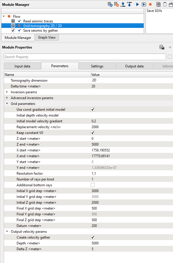
Grid parameters
This group defines the spatial extent and resolution of the tomographic grid, as well as the initial velocity model used to start the inversion. The grid covers the subsurface volume from the datum downward to the specified depth range, and from the lateral extents of the input velocity data. The grid is refined progressively across global iterations, beginning with the initial grid step sizes and converging toward the final (finer) step sizes.
Use const gradient initial model
By default TRUE. If the user prefers a constant gradient keep this option as checked and specify the gradient value in the "Initial model velocity gradient" parameter.
When enabled (default), the inversion begins from a simple 1D velocity model defined by the Replacement velocity at the surface and a constant velocity gradient increasing with depth. This is the recommended starting point when no prior depth velocity model is available. When disabled, the module expects a depth velocity model to be connected as the Initial depth velocity model input, which will be resampled onto the tomographic grid as the starting point.
Initial depth velocity model
Available only when Use const gradient initial model is disabled. Connect an existing depth interval velocity model here to use as the starting model for the inversion. This is useful in iterative workflows, for example when using the output of a previous tomography run or a depth-converted model as the starting point for refinement. The model is automatically resampled onto the current tomographic grid.
Initial model velocity gradient
Specify the velocity gradient value if "Use constant gradient initial model" option is checked.
The velocity increase per meter of depth used to construct the constant-gradient initial model (in m/s per meter). The initial velocity at each depth node is calculated as: Replacement velocity + (gradient x depth). The default is 0.2 (m/s)/m, which corresponds to a typical sedimentary compaction trend. Increase this value for areas with rapid velocity increase (e.g., heavily compacted or carbonate-dominated sequences); decrease it for geologically young, undercompacted sediments.
Replacement velocity
Mention the near surface/replacement velocity of the surface.
The velocity assigned at the datum level (in m/s), used as the starting velocity at the top of the interval velocity model. This value should match the replacement velocity used in the time processing statics application. It also anchors the constant-gradient initial model. The default is 1500 m/s, which is appropriate for marine surveys or near-surface water replacement. For land surveys, adjust this to the near-surface replacement velocity used during processing.
Keep constant V0
By default TRUE.
When enabled (default), the Replacement velocity value at the datum is held fixed and not updated during the inversion. This prevents the near-surface velocity from being altered by the tomographic update, which can be important when the surface velocity is well-constrained from refraction analysis or well data. Disable this option only if you want to allow the inversion to freely update the velocity throughout the entire depth range including the shallowest nodes.
Z start
Define the starting depth value of the interval velocity model
The shallowest depth (in meters) at which the tomographic grid begins, measured from the datum. Typically set to 0 (i.e., starting at the datum level). The default is 0 m. Increase this value if you want to exclude a shallow zone from the inversion, for example if shallow velocities are better constrained by other methods.
Z end
Define the ending depth value of the interval velocity model
The maximum depth (in meters) of the tomographic grid, measured from the datum. The default is 8000 m. Set this to a value slightly deeper than the deepest target of interest. Extending the grid too far below the deepest reliable reflection coverage may produce unconstrained velocities at depth.
X start
The minimum inline coordinate (in meters) of the tomographic grid. This value is automatically populated from the spatial extent of the input RMS velocity gather when data is connected. The default is 0 m. In normal use, leave this at its auto-detected value.
X end
The maximum inline coordinate (in meters) of the tomographic grid. This value is automatically populated from the spatial extent of the input RMS velocity gather when data is connected. The default is 20000 m. In normal use, leave this at its auto-detected value.
Y start
The minimum crossline coordinate (in meters) of the tomographic grid. Applies to 3D mode only. This value is automatically populated from the spatial extent of the input RMS velocity gather when data is connected. The default is 0 m.
Y end
The maximum crossline coordinate (in meters) of the tomographic grid. Applies to 3D mode only. This value is automatically populated from the spatial extent of the input RMS velocity gather when data is connected. The default is 20000 m.
Resolution factor
The factor by which the grid cell size is divided at each global iteration. After the first global pass (which uses the initial grid step), each subsequent pass divides the current grid step by this factor, progressively increasing resolution. The default is 1.1. For example, with an initial X grid step of 3000 m, a resolution factor of 1.1, and 3 global iterations, the X step sizes will be approximately 3000 m, 2727 m, and 2479 m across the three passes. The grid refinement stops when the step size reaches the corresponding final grid step. A larger factor produces a more aggressive resolution increase per iteration.
Number of rays per knot
The number of ray paths traced per grid cell in each spatial direction. Increasing this value subdivides each grid cell and traces additional rays, providing denser ray coverage and potentially improving the accuracy of the velocity update, especially in areas of sparse data. The default is 1 (one ray per knot). Use higher values when the data coverage is uneven and some grid cells are poorly sampled.
Additional bottom rays
When enabled, the module adds extra ray paths at the deepest time level of the velocity model. These additional rays help constrain the velocity at the deepest nodes of the grid, which may otherwise be poorly covered if the reflection data does not extend to the maximum recording time. Disabled by default. Enable this option if the output velocity model shows unconstrained or anomalous velocities at the base of the model.
Initial X grid step
Specify the initial grid step size in X direction
The inline grid spacing (in meters) used at the start of the first global iteration. This is the coarsest inline resolution of the tomographic grid. The default is 3000 m. Set this value to be broadly consistent with the long-wavelength lateral velocity variations expected in your dataset. A value too small relative to the data coverage may produce an ill-conditioned inversion on the first pass.
Initial Y grid step
Specify the initial grid step size in Y direction
The crossline grid spacing (in meters) used at the start of the first global iteration. Applies to 3D mode only. The default is 3000 m. For datasets where crossline coverage is denser or sparser than inline, the Y grid step can be set independently from the X grid step.
Initial Z grid step
Specify the initial grid step size in Z direction
The vertical (depth) grid spacing (in meters) used at the start of the first global iteration. This sets the coarsest depth resolution. The default is 2000 m. A coarser initial Z step is appropriate when the velocity variations are expected to be gradual with depth; use a finer starting step for datasets with sharp velocity contrasts near the surface.
Final X grid step
Specify the final grid step size in X direction
The finest inline grid spacing (in meters) that the grid refinement is allowed to reach. The grid step is reduced by the resolution factor at each global iteration but will never go below this value. The default is 500 m. Set this to the minimum lateral resolution you wish to resolve, keeping in mind that finer grids require sufficient ray coverage to remain well-constrained.
Final Y grid step
Specify the final grid step size in Y direction
The finest crossline grid spacing (in meters) that the grid refinement is allowed to reach. Applies to 3D mode only. The default is 500 m. This value should be consistent with the crossline bin spacing and the available data coverage in the crossline direction.
Final Z grid step
Specify the final grid step size in Z direction
The finest depth grid spacing (in meters) that the depth grid refinement is allowed to reach. The default is 500 m. Use a finer final Z step when you need to resolve sharp velocity contrasts at depth boundaries such as unconformities or salt tops. Avoid setting this finer than can be supported by the temporal resolution of the input RMS velocity data.
Datum
Provide the datum value.
The depth of the processing datum (in meters), which serves as the reference level from which depth imaging is performed. Unlike time-domain processing where migration typically starts from the acquisition topography, depth imaging starts from a flat datum plane. This value must match the datum used during time processing (e.g., in statics application). The default is 0 m. If the input RMS velocity data was computed relative to a non-zero datum (for example, sea level or a topographic datum), set this field accordingly. The module will automatically update this value to the maximum datum elevation found in the data if it exceeds the entered value.
Output velocity params
This group controls whether a regularly sampled depth velocity gather is generated as additional output, and defines the depth range and sampling of that gather. The internal tomographic velocity model (the grid knot-based model) is always produced; these parameters govern only the optional resampled output gather.
Create velocity gather
By default is it FALSE. If the user checks this option, it will generate the output Depth interval velocity model.
When enabled, the module produces a depth-domain velocity gather sampled at regular depth intervals, in addition to the grid-based internal velocity model. This gather can be visualized directly in the 2D viewer as a depth interval velocity volume and can be passed to downstream modules. Disabled by default. Enable this option when you need a regularly sampled depth velocity output for display or for input into migration modules that expect a trace-based velocity model.
Depth
Specify the total length of the output velocity model in terms of depth.
The maximum depth (in meters) of the output velocity gather, measured from the datum. Active only when Create velocity gather is enabled. The default is 8000 m. This should normally match or be slightly less than Z end.
Delta Z
Define the depth sample interval.
The depth sampling interval (in meters) at which the output velocity gather is sampled. Active only when Create velocity gather is enabled. The default is 5 m. A finer sample interval produces a smoother and more detailed output gather but results in a larger output volume. Use a value that is consistent with the expected resolution of the tomographic velocity model and the requirements of downstream processing steps.
Output data
Depth velocity gather
A regularly sampled interval velocity gather in the depth domain. Each trace in this gather contains the interval velocity function versus depth at a surface bin location, sampled at the interval defined by Delta Z. This output is generated only when Create velocity gather is enabled. It can be displayed in the 2D velocity viewer and passed to depth migration modules that accept trace-format velocity inputs.
Depth velocity
The primary output: a depth interval velocity model stored in g-Platform's internal depth velocity format. This is the full tomographic velocity model built from the CRS inversion. It can be connected directly to depth migration modules, used as the initial model for subsequent tomographic refinement passes (e.g., Grid tomography 2D / 3D update), or exported for use in other applications. This output is always produced regardless of the Create velocity gather setting.
Grid velocity
The raw tomographic grid velocity model in g-Platform's internal NIP (Normal Incidence Point) grid format. This output stores the velocity values at the tomographic knot points and is used as input to the Grid tomography 2D / 3D update module for iterative model refinement. It preserves the grid structure of the inversion result and is suitable for connecting directly into the update module to continue building the velocity model with additional constraints such as first-break picks or well data.