Frequency Dependent Noise Attenuation
![]()
![]()
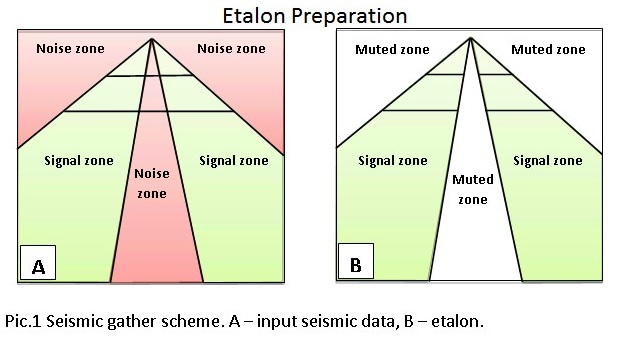
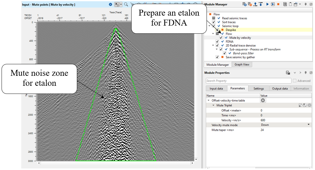
This module uses frequency-dependent and time-variant algorithm where an amplitude threshold values are defined in a trace neighbor area (T-X) for detecting and noise attenuation according to different frequencies and different time windows. The attenuation process consists of two steps – First prepare the etalon (model) and noise attenuation data sets. The etalon should contain only the signal zones, with the noise zone muted. The module estimates the median value of the amplitude spectrum in the sliding windows of the etalon data set, and for each window computes an operator using the threshold value. The procedure attenuates amplitudes whose values exceed the specified threshold.
Output data – 2D/3D seismic gathers in the same sort order as the input data with noise attenuated, and a before and after FDNA difference gather.
![]()
![]()
Input DataItem
Input gather - Two seismic data sets are input to the FDNA module.
The Input gather are 2D/3D seismic gathers in source or receiver sort order. It is better if they are NMO corrected and static corrections have been applied, but for this step we can apply denoise sequence in a soft mode without NMO correction.
Model gather - is the etalon of 2D/3D seismic gathers in source or receiver sort order. The same idea: it is better if they are NMO corrected and static corrections have been applied, but for this step we can apply denoise sequence in a soft mode without NMO correction.
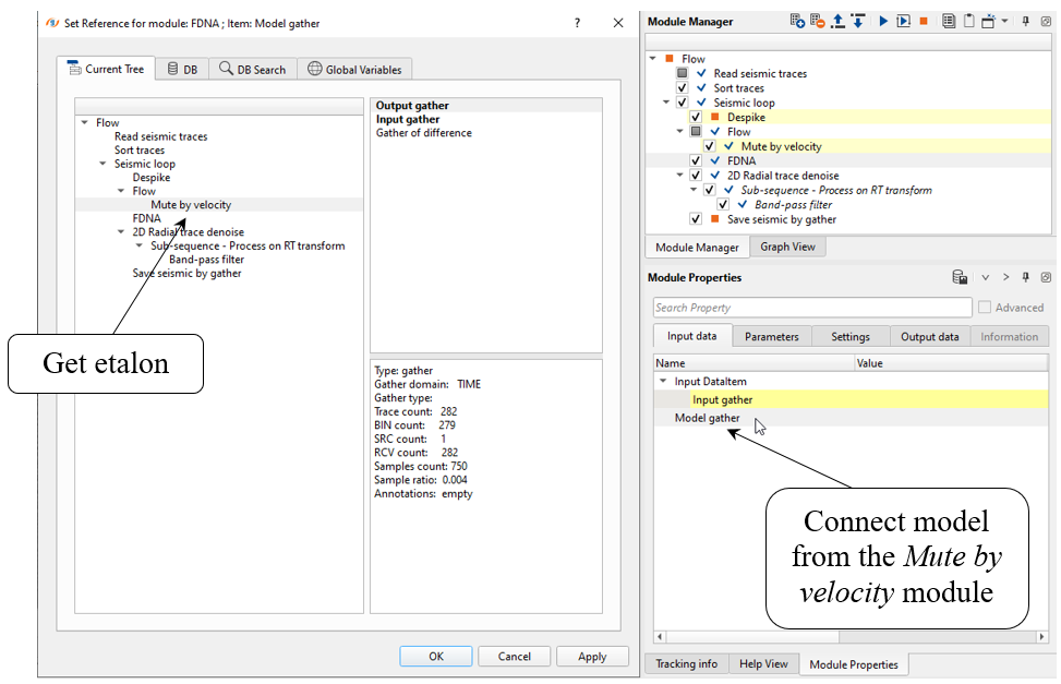
Link to input etalon seismic gather with internal and external noise muted.
This module use the etalon for creating a correction filter for the input seismic data.
The user must prepare the etalon before running FDNA.
![]()
![]()
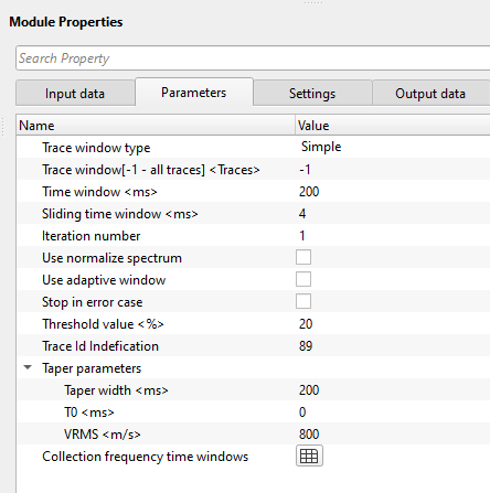
Trace window type { Simple, Time dependent } - trace window or horizontal window is used to attenuate the noise locally. There are two types of trace windows are available for the drop down menu.
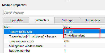
Simple - it works like normal trace window where the user should provide number of traces to be considered as a trace window.
Time dependent - as the name suggest, different number of traces will be considered at different times. As we know that FDNA is used for attenuating ground roll and it (ground roll noise) increases with the increase in time. So time dependent trace window will be a good option to attenuate the ground roll effectively.
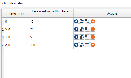
Trace window[-1 - all traces] - number of adjacent traces used for comparing the spectrum of both input and model. These traces are used for the sliding window and also used for local attenuation.
•Default: -1 (all traces)
•Range: from 1 to max traces in the input gather
Time window - the vertical analysis window length (in seconds) used to estimate the local amplitude spectrum. Default: 0.2 s (200 ms). The taper zone between adjacent windows is one quarter of this length.
A longer time window captures more cycles of low-frequency noise (such as ground roll), which produces a more stable spectral estimate and stronger attenuation of that noise. A shorter window is better for resolving rapid time-variant changes in the noise character, but may produce a noisier threshold estimate. For most ground-roll attenuation applications, values between 0.1 s and 0.5 s are appropriate. The time window should be at least two full cycles of the lowest frequency to be attenuated.
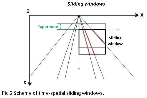
Sliding time window - amount to advance the sliding time window each shift
Specifies how much the analysis window steps forward along the time axis between successive processing positions. The default is 0.004 s (4 ms), which matches a typical seismic sample interval. Smaller values produce smoother noise attenuation at the cost of longer computation time. Values larger than the Time window will leave gaps in the processing and are not recommended.
Time window type { Constant time, Parabolic with constant velocity, Parabolic with velocity model } - controls the shape of the vertical analysis window applied across the gather.
Three options are available. Constant time (default) applies a flat horizontal time window of the same length at all offsets. Parabolic with constant velocity curves the window hyperbolically using a single user-defined velocity, which is useful when a representative NMO velocity is known for the noise zone. Parabolic with velocity model uses a full velocity model item to vary the window curvature with time and position, giving the most accurate result when velocity varies laterally or with depth. When either parabolic option is selected, an additional velocity input becomes available.
Iteration number - defines the number of iterations to perform. The more iterations, the longer the run time.
Default: 1. Each iteration feeds the output of the previous pass back into the filter as the new input, progressively removing more noise energy. A single iteration is appropriate for most data sets. Use 2 to 3 iterations when the noise is particularly strong or when the etalon (model) is imperfect. More than 3 iterations rarely yields additional benefit and significantly increases processing time.
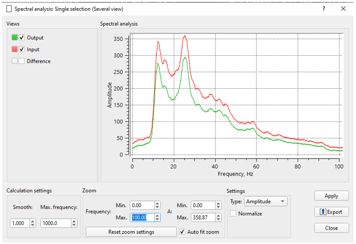
Use normalize spectrum - by default, FALSE (Unchecked). This option is used to normalize both input and model gathers to compare the spectrum. It is very useful when there is a huge amplitude difference.
When enabled, both the input gather and the model gather are normalized before their spectra are compared. This makes the comparison amplitude-independent, so the filter focuses purely on spectral shape differences rather than energy level differences. Enable this option when the model gather has been created from a different gain or amplitude scaling than the input, or when there is a large overall amplitude imbalance between the two data sets.
Use adaptive window - by default, FALSE (Unchecked). If TRUE (Checked), it will adjust the time window size automatically depending on the local signal characteristics. Low-frequency content receives a larger time window, and high-frequency content receives a smaller time window.
Enabling the adaptive window allows the algorithm to automatically tune the analysis window length to the dominant frequency at each time-trace location. This can improve noise attenuation on data where the signal bandwidth changes significantly with time, for example when high-frequency signal attenuates with depth and low-frequency noise such as ground roll dominates the shallow portion. Leave this option off for a first-pass test; enable it if the fixed window produces over- or under-attenuation at particular time ranges.
Stop in error case - stops the processing if the module encounters any error during execution. By default, FALSE (Unchecked).
When enabled, the module checks whether any output sample that was non-zero in the input has been set to zero in the output. If such a discrepancy is detected, processing halts and an error message identifies the affected time sample. Enable this option during quality control testing to catch unexpected results early. For routine production runs, leave this option unchecked so that the job continues even if a single gather produces an anomalous result.
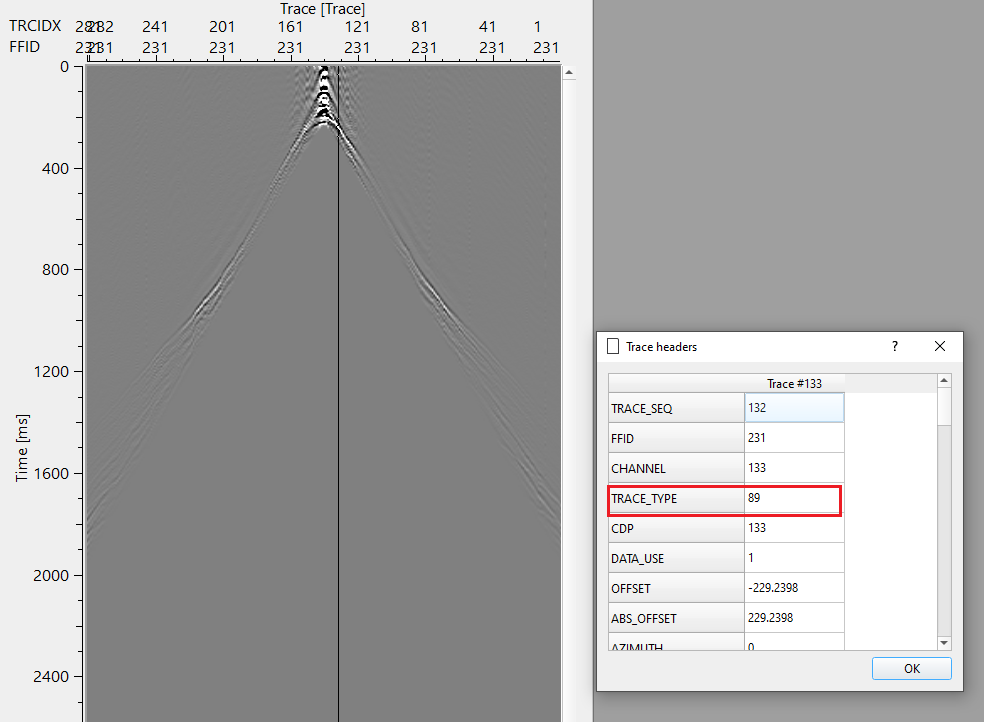
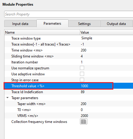
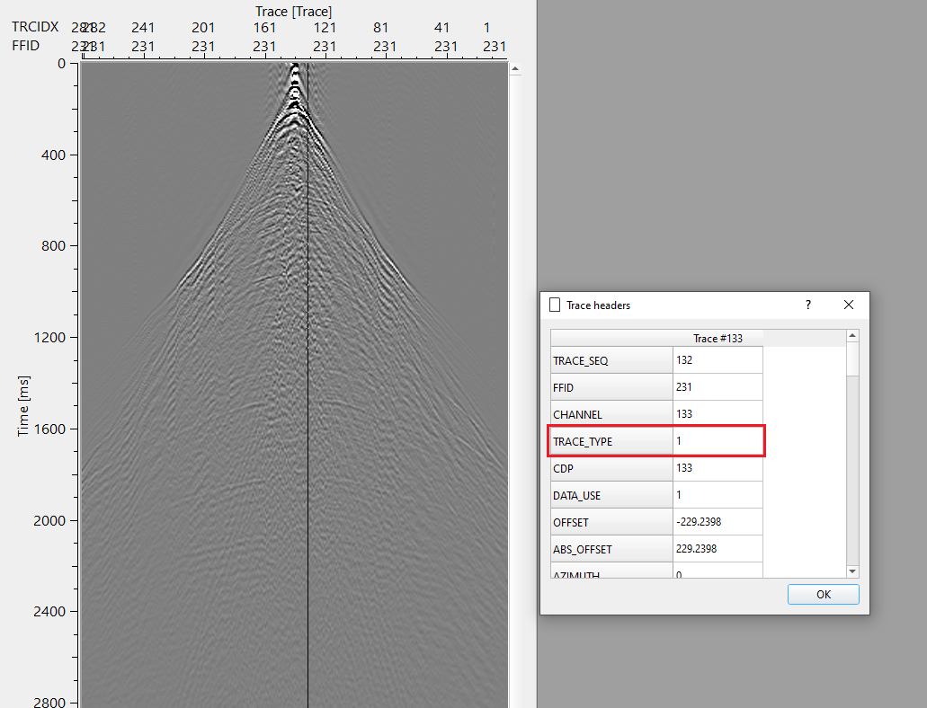
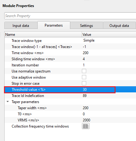
Threshold value - defines how much difference between input and output is acceptable. If the ratio of non-zero samples in the etalon to non-zero samples in the input falls below this value, the etalon is considered invalid and is replaced by the input gather itself. Default: 0.3 (30%).
This parameter acts as a validity check on the model gather. It compares the proportion of non-zero samples in the etalon against those in the input. If the etalon has been over-muted (too many zeros relative to the input), the model is considered unreliable and the module substitutes the raw input as the reference. The default value of 0.3 means that if less than 30% of the etalon samples are non-zero compared to the input, the etalon is rejected. Raise this value if you want the algorithm to be stricter about requiring a valid etalon; lower it if the etalon is expected to have many muted zones.
Trace Id Identification - specifies the trace type identifier assigned to gathers when the etalon is detected as invalid. Default: 89.
When the etalon validity check (controlled by Threshold value) fails for a gather, the module marks each output trace with the TRID (trace identification) header value specified here, changing it from the standard value of 1. This allows downstream QC processes to identify and flag gathers that were processed without a valid model. In most workflows this parameter can be left at the default value of 89.
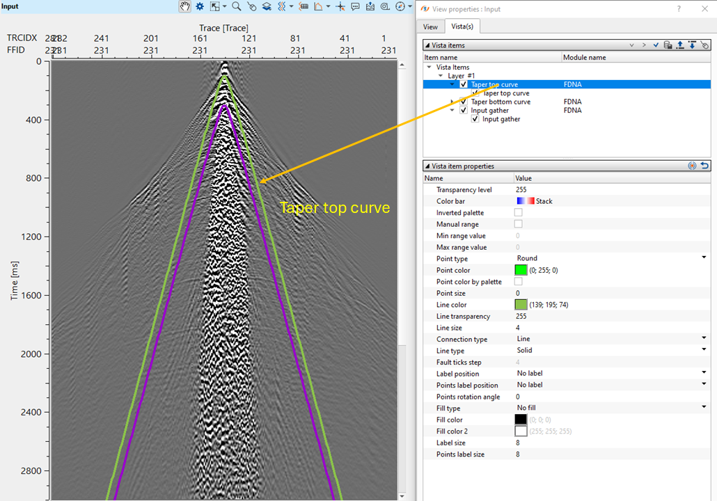
Taper parameters - taper is helpful in smooth transitioning of the processed data by not creating any sharp boundary, edge effects or artifacts.
The taper is applied to the near-time (shallow) portion of the output gather to blend the unprocessed original data with the FDNA-filtered data. The taper zone is defined by a hyperbolic curve computed from the T0 and VRMS values, and its transition width is set by the Taper width parameter. Within the taper zone, samples are blended linearly between the raw input (at the top of the taper) and the fully filtered output (at the bottom). Taper curves are displayed as overlays on the gather view and update interactively as parameter values change.
Taper width - there are two taper curves drawn based on the Vrms value. One taper curve will be the top and the other one will be the bottom curve. In between these two taper curves, the user should provide a taper width for smooth transitioning of the data to avoid any sharp boundaries or edge effects.
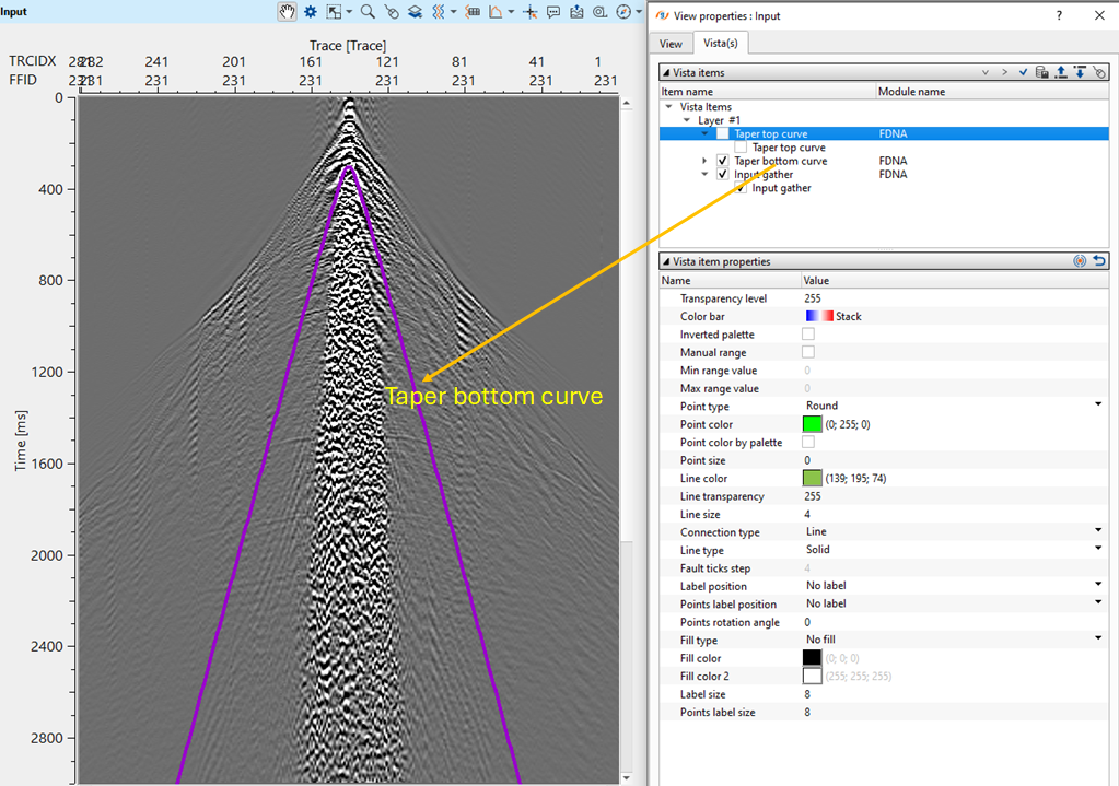
T0 - specify the central time for the taper curves to start with. By default, 0 ms. Based on this value, both the taper curves starts symmetrically on the both sides of the shot gather (for Split spread).
VRMS - specify the velocity value for the taper curves. By default, 1500 m/s.
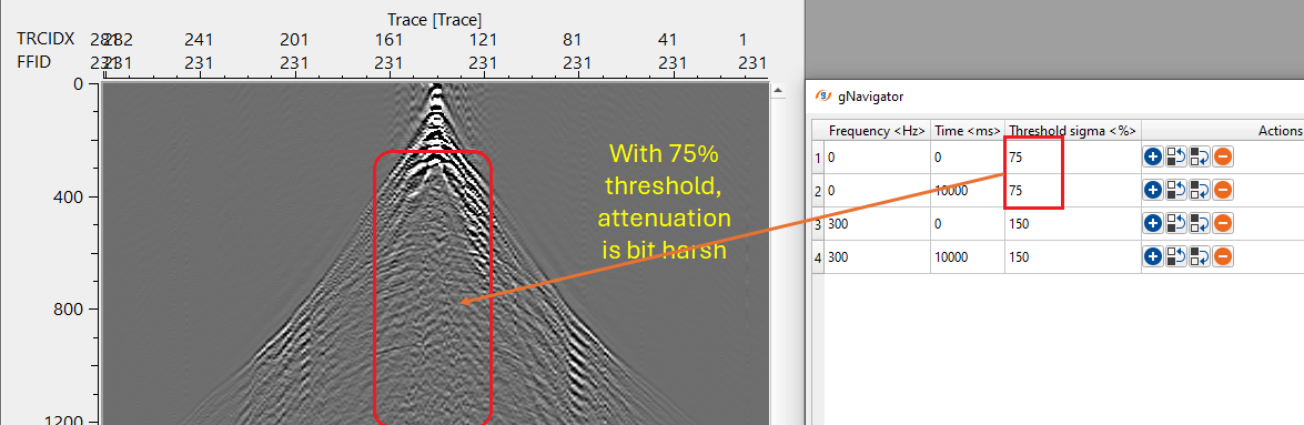
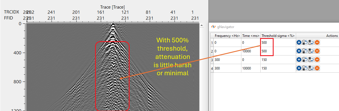
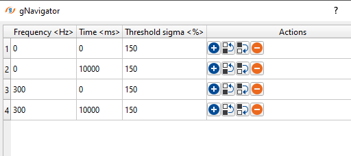
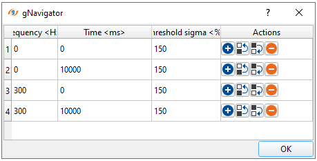
Collection frequency time windows - this section defines the time-frequency pairs that control noise attenuation at different time and frequency bands. These three parameters — Frequency, Time, and Threshold sigma — together define the attenuation behavior across the entire data set.
Each row in the collection specifies a (Frequency, Time, Threshold sigma) triplet. The algorithm interpolates the threshold sigma value between these control points across the full time and frequency range. By adding multiple rows you can apply stronger attenuation at the frequencies and times where noise is dominant, and gentler attenuation where signal is important. For example, use a larger threshold sigma at shallow times or low frequencies to protect near-surface reflectors from being attenuated together with the noise. The collection must span a frequency range of at least 5 Hz, otherwise the module will report an error. The default collection covers the full frequency range (0 to 300 Hz) over the full time range (0 to 10 s) with a uniform threshold sigma of 1.5.
• Frequency – frequency for attenuation
Default: 0 (Hz)
Range: from 0 to max sampling frequency (Hz)
•Time – time value for threshold
Default: 0 (Hz)
Range: from 0 to max trace length(ms)
•Threshold sigma (%) – the limiting parameter for calculating threshold values to attenuate excessive amplitudes
Default: 1.5 (sigma multiplier);
Range: from 0 to 99999. Lower values apply stronger attenuation; higher values preserve more signal energy.
![]()
![]()
Auto-connection - By default, TRUE(Checked).It will automatically connects to the next module. To avoid auto-connect, the user should uncheck this option.
Bad data values option { Fix, Notify, Continue } - This is applicable whenever there is a bad value or NaN (Not a Number) in the data. By default, Notify. While testing, it is good to opt as Notify option. Once we understand the root cause of it, the user can either choose the option Fix or Continue. In this way, the job won't stop/fail during the production.
Notify - It will notify the issue if there are any bad values or NaN. This will halt the workflow execution.
Fix - It will fix the bad values and continue executing the workflow.
Continue - This option will continue the execution of the workflow however if there are any bad values or NaN, it won't fix it.
Calculate difference - This option creates the difference display gather between input and output gathers. By default Unchecked. To create a difference, check the option.
Number of threads - One less than total no of nodes/threads to execute a job in multi-thread mode. Limit number of threads on main machine.
Skip - By default, FALSE(Unchecked). This option helps to bypass the module from the workflow.
![]()
![]()
Output DataItem
Output gather - the primary output of the FDNA module: the input gather with frequency-dependent noise attenuated.
The output gather has the same trace count, sample count, and sort order as the input. Amplitudes that exceeded the frequency-dependent threshold relative to the model gather have been suppressed, while samples within the taper zone are blended linearly with the original input. Connect this output to the next module in the processing sequence.
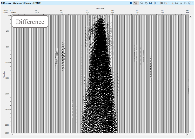
Gather of difference - generates the difference gather showing what was removed by the noise attenuation process.
This gather contains the sample-by-sample difference between the input and the output (Input minus Output). It is available only when the Calculate difference option is enabled in the Settings tab. Review this gather to verify that only noise has been removed and that no coherent signal energy appears in the difference. Coherent energy in the difference gather is an indicator that the threshold values are set too aggressively.
The FDNA module does not define any custom action buttons. All processing is performed by executing the module in the standard workflow. Use the taper curve overlays in the gather view to visually verify the taper zone before running the full dataset.
![]()
![]()
Carefully prepare the etalon (model) data, try to mute the high amplitude zones and include the signal zones. Control the noise attenuation by using the threshold parameters and the ability to specify the thresholds in a time variant manner and by frequency.
This procedure is more effective in the first steps of the seismic data processing flow when noise zones still have high amplitudes. The input seismic data should not be amplitude normalized.Create the Etalon (model) in a Seismic loop.
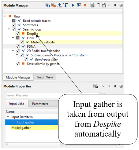
Seismic loop makes automatic connections between all modules in a sequence under that seismic loop and the user cannot disconnect them. In this case, we need to use an additional “Flow” module inside of the Seismic loop for etalon preparation. Put the mute modules into a “Flow” inserted into the Seismic loop and then connect the output muted data to the Model gather field of the Input data tab of the FDNA module. The Input gather on the Input data tab will be automatically connected to the previous module in the Seismic loop processing flow.
Let's have a look at the example workflow.
Seismic loop makes automatic connections between all modules in a sequence under that seismic loop and the user cannot disconnect them. In this case, we need to use an additional Flow module inside of the Seismic loop for etalon preparation. Put the mute modules into a Flow inserted into the Seismic loop and then connect the output muted data to the Model gather field of the Input data tab of the FDNA module. The Input gather on the Input data tab will be automatically connected to the previous module in the Seismic loop processing flow.
Create an etalon for FDNA by using Mute by velocity module:
Next, we need to connect input Model gather (etalon) with output from the Mute by velocity module:
Input data is taken from Despike:
FDNA parameters:
Collection frequency time windows:
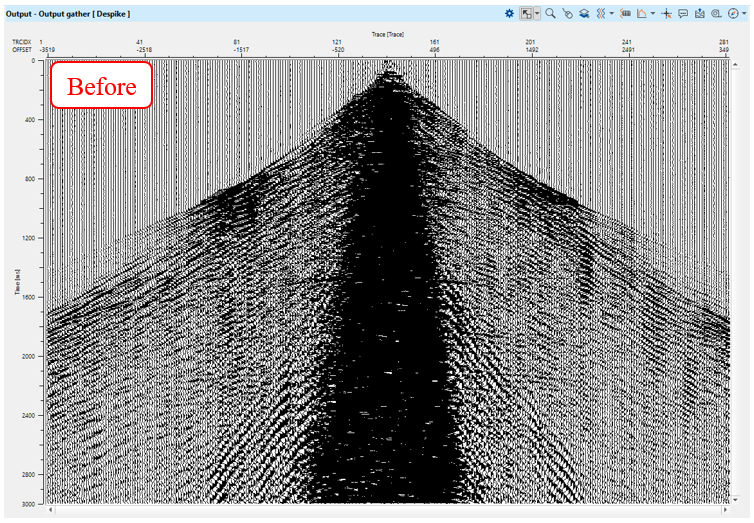
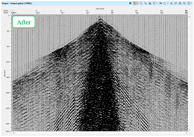
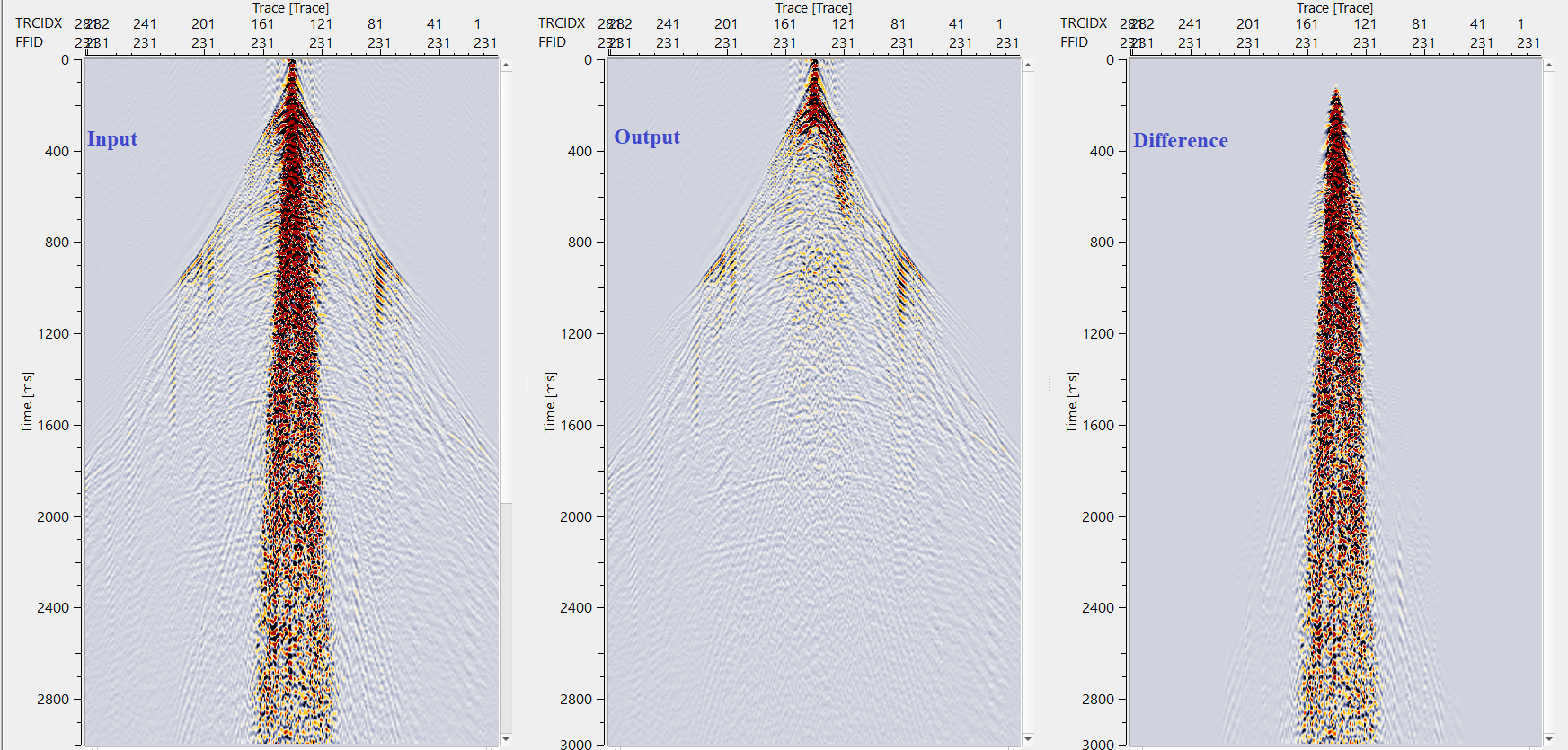
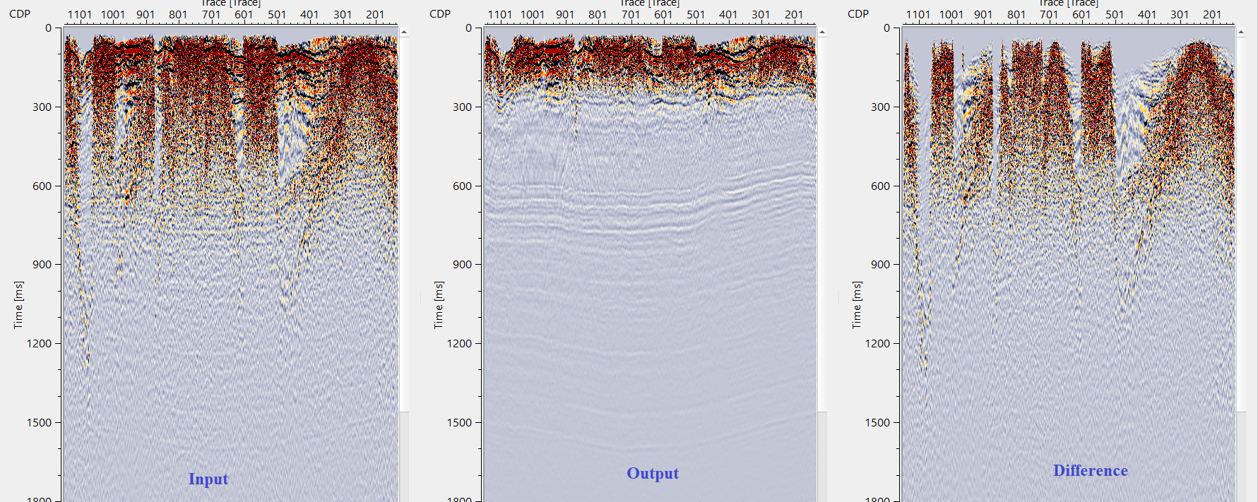
Execute FDNA and check the results, source gathers before - after - difference:
![]()
![]()
There are no action items available for this module so the user can ignore it.
![]()
![]()
YouTube video lesson, click here to open [VIDEO IN PROCESS...]
![]()
![]()
Yilmaz. O., 1987, Seismic data processing: Society of Exploration Geophysicists
Shettar A., 2019, F-K Filtering for Seismic Data Processing
 If you have any questions, please send an e-mail to: support@geomage.com