Analyzing amplitude and frequency spectrum(s) of the input data
![]()
![]()
Fast Spectral Analysis computes the amplitude spectrum of one or more seismic gathers and displays the result as a frequency-versus-amplitude plot in real time. It is a lightweight QC and diagnostic tool used to assess the bandwidth of a dataset, identify frequency-domain noise, evaluate the effectiveness of filters or deconvolution, and guide parameter selection for processing steps that are sensitive to spectral content.
For each connected gather, the module applies a Fast Fourier Transform (FFT) over the specified time and trace window and accumulates the amplitude spectrum across all selected traces. The result is optionally smoothed and then displayed using the chosen normalization scale. Multiple gathers can be connected simultaneously, each producing its own spectrum curve on the same plot for direct comparison.
Unlike the full Spectral Analysis module, this module does not modify the data — it is a read-only display tool. The analysis window can be set by entering time and trace limits numerically, or by drawing a rubber-band rectangle directly on the seismic display panel.
![]()
![]()
GGather collection - add the input data gather collection by clicking on the  icon.
icon.
This collection holds one or more gathers to be analyzed. Connect any pre-stack or post-stack gather — common-shot, common-receiver, CMP, or stack section. Each gather added to the collection produces a separate spectrum curve on the output frequency-amplitude plot, enabling direct side-by-side comparison of spectral content across different data sets, processing stages, or offset classes. At least one gather must be connected before running the module.
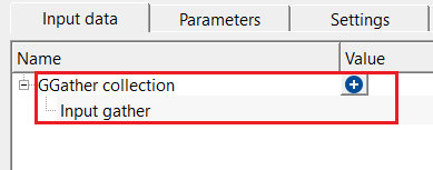
Input gather - connect/reference to the input gather where the user perform the spectral analysis.
Each entry in the GGather collection represents one gather connection. The gather is displayed in the seismic panel (Input data view) and its spectrum is computed and plotted in the frequency-amplitude panel (Frequency-Amplitude/DB view). Any type of seismic gather is accepted; the module is read-only and does not alter the data.
![]()
![]()
Smooth window - smooths spectrum curve. Higher values produce smoother spectrum. By default, 1
Controls the width (in Hz) of the sliding averaging window applied to the amplitude spectrum after FFT. Internally the window is converted to a number of frequency samples equal to the window width divided by the frequency resolution. A value of 1 Hz (default) applies only light smoothing and preserves fine spectral detail. Increase this value to 5–20 Hz to reduce short-scale oscillations in the spectrum curve and make broad-band trends easier to read. Setting the value to 0 disables smoothing entirely and shows the raw FFT spectrum, which is useful when looking for sharp notches or narrow-band noise.
Max frequency - specify the maximum frequency should be considered. By default, 500 Hz.
Sets the upper frequency limit (in Hz) of the displayed spectrum. The module truncates the FFT output at this frequency so that only the range from 0 Hz to the specified maximum is plotted. The default value of 500 Hz covers the full usable bandwidth for most seismic acquisition settings. Reduce this value to zoom in on the low-frequency portion of the spectrum — for example, set 150 Hz for a typical land survey to focus on the signal band and suppress the high-frequency visual noise tail.
Normalization mode { Normalized, Db, Amplitude } - specifies how spectral amplitudes are scaled for display and comparison. By default, Amplitude.
This setting controls how the vertical axis of the frequency-amplitude plot is scaled. Choose the mode that best suits the analysis goal:
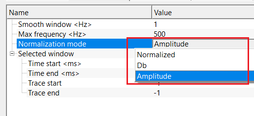
Normalized - scales amplitudes to a peak value of 1.0. All spectrum curves in a multi-gather comparison share the same vertical scale, so differences in bandwidth and shape are immediately visible. The absolute amplitude level is removed, making this mode suitable for comparing the spectral shape between pre- and post-processing stages or between different datasets.
Db - converts amplitudes first to a normalized peak-of-1 scale, then to decibels using 20 * log10(amplitude). This logarithmic display compresses the dynamic range and makes weak-signal components — such as low-amplitude noise tails or spectral roll-off — visible alongside the dominant signal. Use this mode to evaluate noise floor, filter rejection quality, and the effective bandwidth at a chosen dB level below peak.
Amplitude - displays the raw linear amplitude spectrum without any normalization. Absolute spectral energy levels are preserved, so spectra from different gathers can be compared on a common scale. Use this mode when evaluating the true energy difference between two processing results, for example, before and after noise attenuation.
Selected window - this section deals with user inputs. User can choose specific time and traces to analyze the spectrum response.
These four parameters define the sub-window of the gather used for spectral computation. Only the samples and traces within the window are included in the FFT. This lets you focus the spectral analysis on a specific target zone — for example, a shallow reflection package or a known noisy interval — rather than using the entire trace length. The window boundaries can also be set interactively by drawing a rubber-band rectangle directly on the seismic panel: left-click and drag to define the corners, and release to confirm the selection. The parameter fields update automatically when you draw a window interactively.
Time start - specify the starting time window to perform the spectral analysis. By default, -1.
The start time of the analysis window in seconds. A value of -1 (default) means the analysis begins at the first sample of the trace (time zero or the recorded start time). Set an explicit time value to restrict analysis to a particular time interval, such as a target reflection zone.
Time end - specify the ending time window to perform the spectral analysis. By default, -1.
The end time of the analysis window in seconds. A value of -1 (default) means the analysis extends to the last sample of the trace (full record length). Narrowing the window to a specific time range improves the spectral estimate for that zone and reduces contributions from unrelated signal or noise outside the interval of interest.
Trace start - provide the starting trace to consider in the spectral analysis. By default, -1.
The zero-based index of the first trace to include in the spectrum. A value of -1 (default) means start from trace 0 (the first trace in the gather). The spectra of all included traces are accumulated into a single composite spectrum, so restricting the trace range allows you to analyze a spatial sub-region of the gather — for example, a specific offset class or a group of near-offset traces.
Trace end - provide the ending trace number to consider in the spectral analysis. By default, -1.
The zero-based index of the last trace to include in the spectrum. A value of -1 (default) means use all traces up to the last trace in the gather. Together with Trace start, this defines the lateral extent of the analysis window. If the value entered exceeds the actual number of traces, the module automatically clips it to the last available trace.
![]()
![]()
Number of threads - One less than total no of nodes/threads to execute a job in multi-thread mode. Limit number of threads on main machine.
Sets the maximum number of CPU threads used for parallel computation when multiple gathers are connected. Because Fast Spectral Analysis is a lightweight operation, the default thread count is sufficient for most use cases. Reduce this value if you need to reserve CPU resources for other concurrent processes on the same machine.
Skip - By default, FALSE(Unchecked). This option helps to bypass the module from the workflow.
When checked, the module is bypassed entirely and the workflow continues without computing any spectra. This is useful during workflow development when you want to temporarily disable the spectral display without deleting its configuration. By default this option is unchecked (the module executes normally).
![]()
![]()
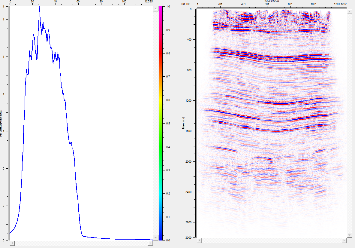
Fast Spectral Analysis is a display-only module and produces no output data items that can be connected to downstream modules in a workflow. All results are shown interactively in the two built-in display panels described below and are not written to disk. To persist spectral results for documentation or further processing, use a screenshot of the frequency-amplitude panel or export data via the full Spectral Analysis module.
Frequency-Amplitude/DB view — the primary output panel. Displays one spectrum curve per connected gather, plotted as frequency (Hz) on the horizontal axis versus amplitude (or dB) on the vertical axis. All curves share the same axes, enabling direct visual comparison. The selected analysis window is reflected in the spectrum immediately after re-executing the module.
Input data view — a standard seismic wiggle/color display of the connected gather. The rubber-band selection rectangle (Selected area overlay) is drawn on this panel to define the analysis window interactively.
Fast Spectral Analysis has no custom action buttons. The module does not expose any verbs such as "Solve" or "Update" because the spectrum is recomputed automatically each time the module is executed or its parameters are changed. Interaction with the analysis window is performed directly in the seismic display panel using the rubber-band selection described under the Selected window parameter group above.
![]()
![]()
In this example workflow, we are reading a stack section as an input gather. As we know, any shot gather (common source/receiver/bin) or stack can be used to perform the spectral analysis.
A typical QC workflow connects two gathers to the GGather collection — for example, the input data before filtering and the output data after filtering. Both spectrum curves are then displayed on the same plot so the effect of the filter on the frequency content can be evaluated visually. Set the Normalization mode to Normalized to compare shapes, or to Db to see how much energy was removed in the noise band.
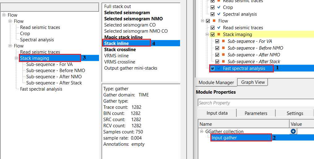
Adjust the parameters as per the input data requirement. We are executing this workflow with the default parameters.
![]()
![]()
There are no action items available for this module so the user can ignore it.
![]()
![]()
YouTube video lesson, click here to open [VIDEO IN PROCESS...]
![]()
![]()
Yilmaz. O., 1987, Seismic data processing: Society of Exploration Geophysicist
 * * * If you have any questions, please send an e-mail to: support@geomage.com * * *