Gather conditioning
Since we calculate and apply migration velocity and Thompson's parameters there is still some under-corrections on far offsets that we need to flatten. g-Platform system contains special module for that task called RMO by picking (manual or auto).
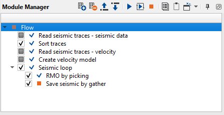
Read seismic traces - seismic data. Load seismic data set after migration 0400_APSTM.
Sort traces. sorting by CDP - OFFSET:
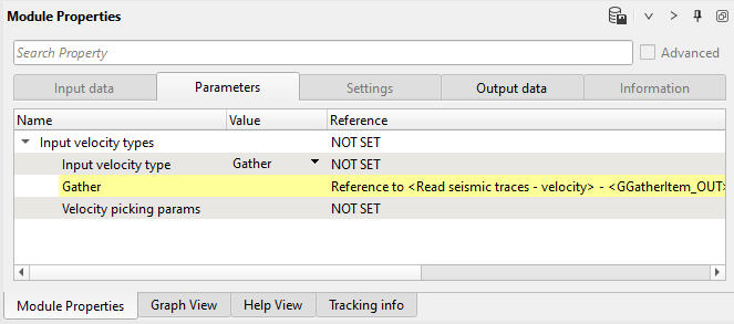
Read seismic traces - velocity. Load gather migration velocity.
Create velocity model. Convert gather migration velocity into velocity model format.
Parameters:
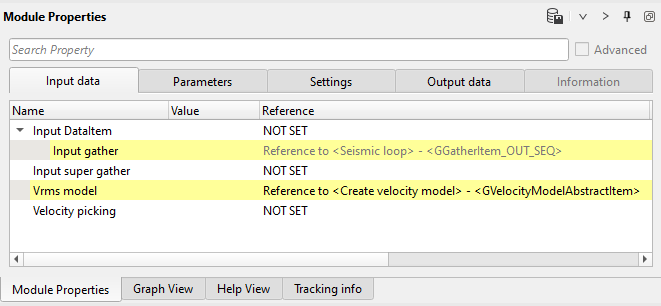
RMO by picking. This module transforms seismic calculates velocity correction and corrects velocity model using residual moveout correction.
Define input data items and parameter:
Input data:
Switch off auto picker mode, because we are going to use manual picking of RMO.
Parameters:
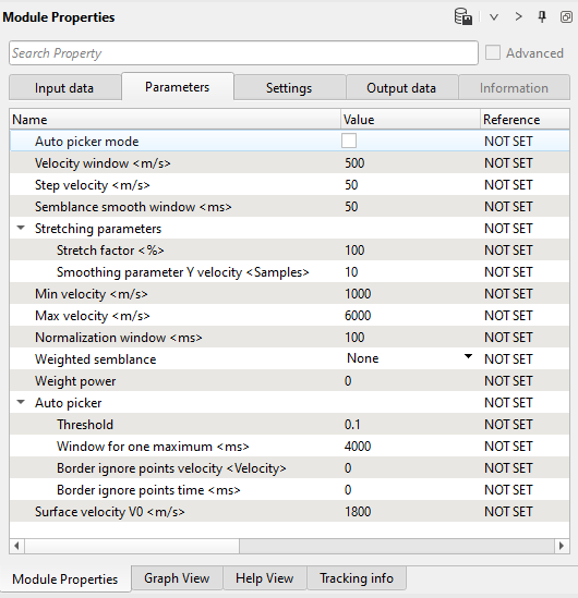
Open all vista groups. Perform manual RMO picking on Velocity Analysis window and check on Output CIG gather. Input window does have time arrival curves. We need to pick CIG points with increment (i.e. 500 meters):
=================================
And add all necessary modules, connect all input and output data (trace headers, SEG-Y handlers):
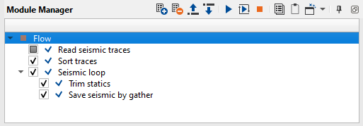
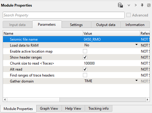
1) Read seismic traces. Load seismic data set 0459_RMO.
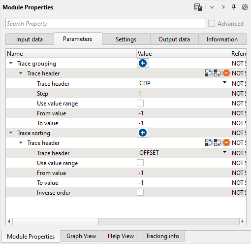
2) Sort traces. Here we need to sort seismic traces for Seismic loop, add Sort traces module and set CDP-OFFSET headers for sorting:
3) Seismic loop. Connect trace headers vector (Input sorted headers) from the Sort traces module output and seismic (Input SEG-Y data handle) from Read seismic traces.
4) Trim statics. module can be used inside Stack Imaging or Seismic loop modules in two main types: Constant time and Time variant.
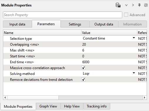
In Constant time type we apply one static shift for each trace inside gather. Main parameters in this mode is:
•Max shift <ms> - max shift for static correction;
•Start time <ms> - start time for static correction;
•End time <ms> - end time for static correction;
•Massive cross-correlation approach (true or false) – default calculation use cross-correlation between each trace of gather and stack trace, massive cross-correlation approach use cross-correlation between each trace of gather with other traces; this method more intense but theoretically more precise;
•Solving method – Gauss-Seidel or Lsqr (least-squares);
•Remove deviations from trend detection (true or false) – remove median static deviation from static correction.
In Time variant type we apply multiple static shift for each trace inside gather correspond to windows for static correction. Main parameters in this mode is:
•Overlapping <ms> - overlapping between windows to prevent static glitches between adjacent windows;
•Massive cross-correlation approach (true or false) – default calculation use cross-correlation between each trace of gather and stack trace, massive cross-correlation approach use cross-correlation between each trace of gather with other traces; this method more intense but theoretically more precise;
•Solving method – Gauss-Seidel or Lsqr (least-squares);
•Remove deviations from trend detection (true or false) – remove median static deviation from static correction;
•Time variant – a table that allows you to set window borders and maximum shifts for them.
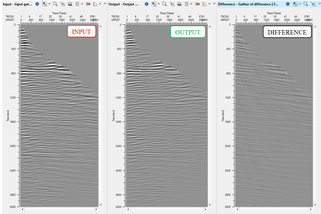
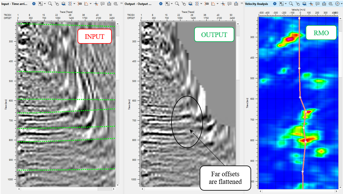
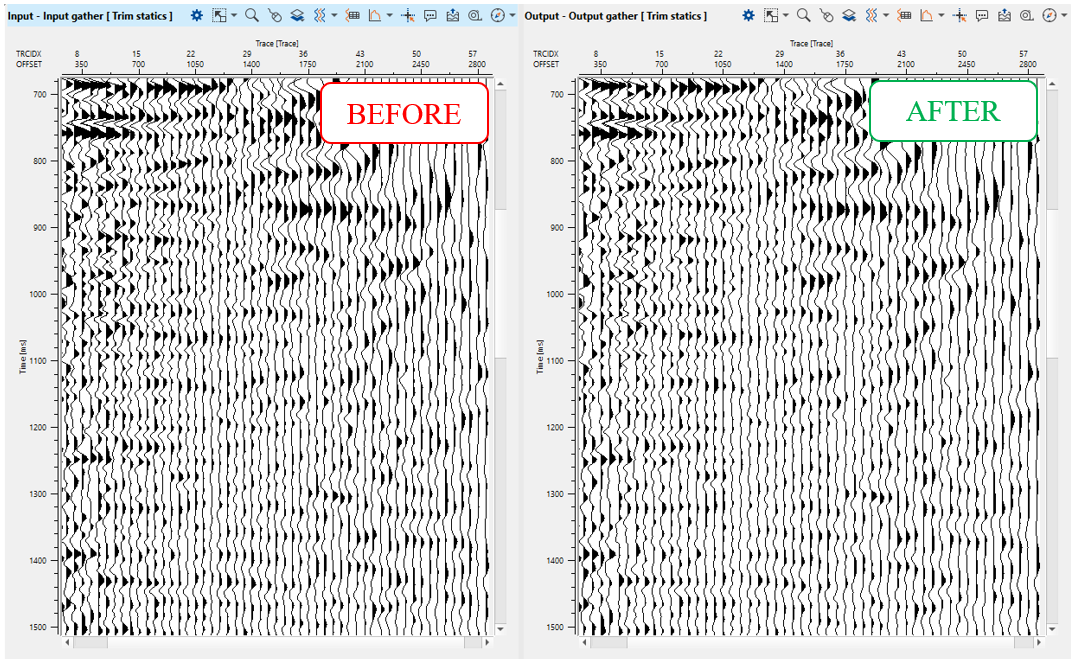
Execute the module and check the results: CIG gather before and after trim static. Obviously, that result is uncertain, therefore we can use in production or leave it as test:
===================================
Additional denoise step performs residual noise attenuation that remained (linear, random, multiple diffraction, etc.) and appear (aliasing, artifacts, etc.) during the entire seismic processing sequence. Use this noise attenuation with caution, because it may be harsh denoise workflow, so all the parametrization and number of iteration you are able to change.
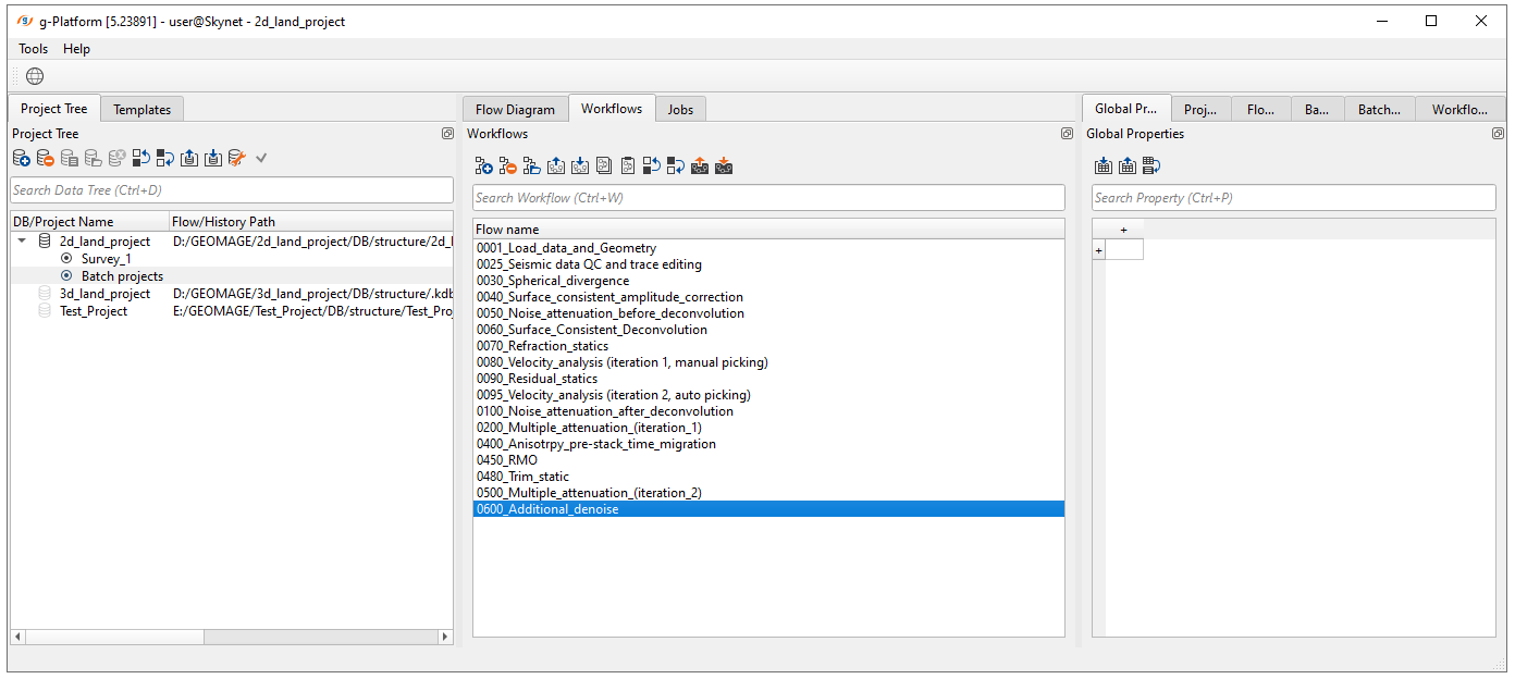
Create a new workflow 0600_Additional_denoise:
Add all necessary modules to the workflow:
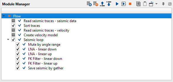
1. Read seismic traces - seismic data - load traces after de-multiples (2-nd iteration)
2. Sort traces - sort traces by CMP
3. Read seismic traces - velocity - load migration velocity
4. Create velocity model - convert seismic gather velocity into a velocity model format
5. Seismic loop - process every sorted gather in a loop (one by one)
6. Mute by angle range - remove far offset stretches
7. LNA - linear down - residual linear wave and allias attenuation iteration 1
8. LNA - linear up - residual linear wave and allias attenuation iteration 2
9. FK Filter - linear up - residual linear wave and allias attenuation iteration 3
10. FK Filter - linear down - residual linear wave and allias attenuation iteration 4
11. Save seismic by gather - save CIG gathers after denoise
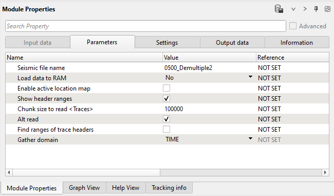
1) Read seismic traces - seismic data. Load seismic data set after migration 0500_Demultiple2.
Parameters:
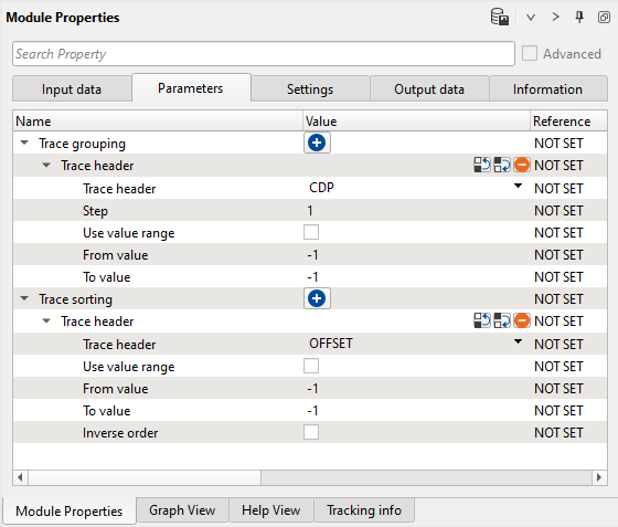
2) Sort traces. Here we need to sort seismic traces for Seismic loop. Add Sort traces module and set CDP and OFFSET header for sorting as it is shown below:
Parameters:
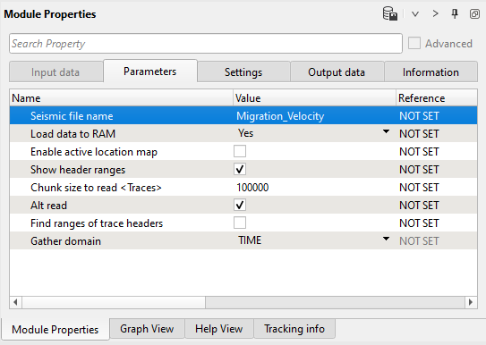
3) Read seismic traces - velocity. Load gather migration velocity.
Parameters:
4) Create velocity model. Convert gather migration velocity into velocity model format.
Parameters:
3) Seismic loop. Connect trace headers vector (Input sorted headers) from the Sort traces module output and seismic (Input SEG-Y data handle) from Read seismic traces.
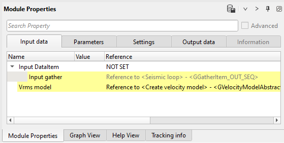
4) Mute by angle range module. Define input data items (seismic + velocity).
Input data:
Parameters:
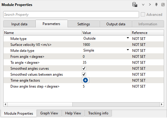
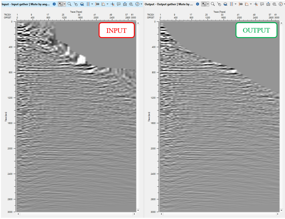
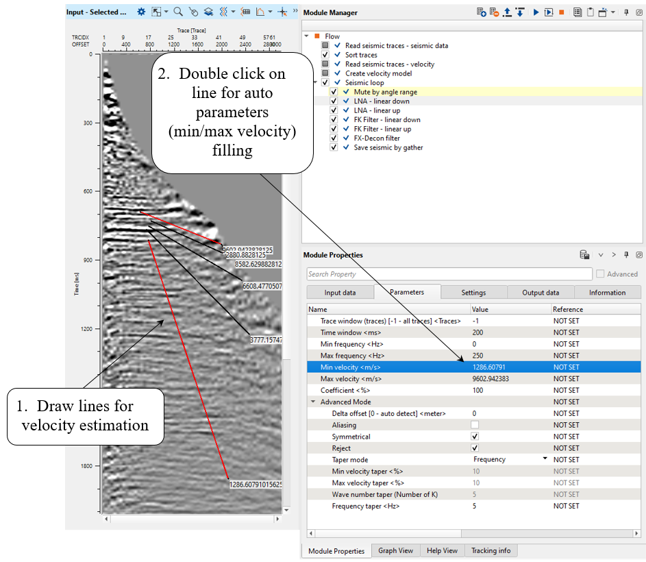
Then, open all vista windows, analyze far offsets and create a mute function for cutting useless stretches on far offsets. Look at angle vista window, obviously we can use 35 degrees for saving:
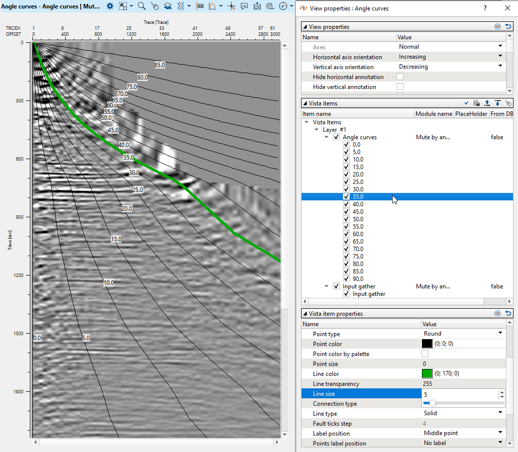
Check out CIG gather:
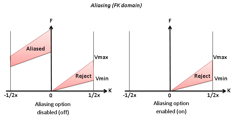
5) LNA - linear down - Linear noise attenuation. This procedure computes linear wave (noise) attenuation in the frequency-wave number (FK) domain in the local sliding time-spatial windows. Input seismic gathers transformed from the time spatial (TX) domain to the FK domain. Horizontal waves have infinite apparent velocity and shown as vertical lines in the FK domain. Vertical waves have zero apparent velocity and shown as horizontal lines in the FK domain. This definition uses for attenuate linear waves.
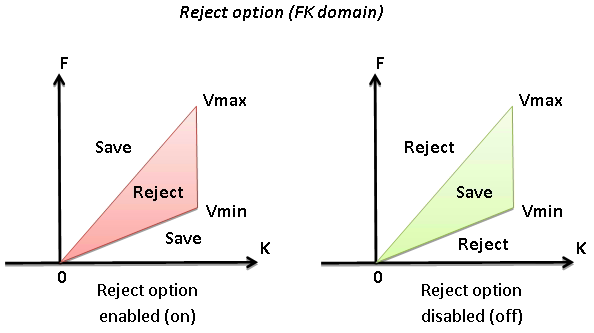
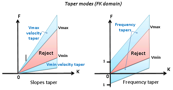
Zones for rejection (reject option is switch on) or saving (reject option is switch off) in the FK domain limited by velocity lines and their slopes must be defined. The slope is apparent velocity in the spatial time (T, X) domain. There is a filter of two velocities (min, max), taper’s bound defined by two mutually exclusive parameters there are frequency and slopes.
We named (commented) this module as linear down, where down means conventional linear wave goes up-down from zero near to far offset.
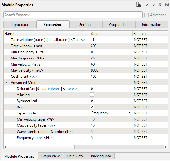
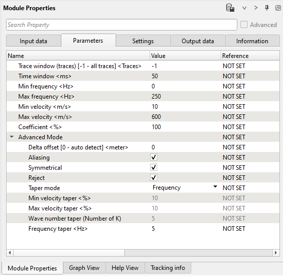
Parameters:
Settings:
Parameters definition:
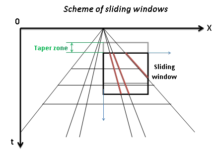
Trace window (traces) [-1 - all traces]
Number of traces for sliding window. This window used for local attenuation. Taper zone between sliding windows is ¼ of trace window
•Default: -1 (all traces)
•Range: from 1 to max traces in the input gather
Time window
Milliseconds for sliding window. This window used for local attenuation. Taper zone between sliding windows is ¼ of time window
• Default: 200 (ms)
• Range: from 1 to max trace length
Min frequency
Minimum frequency for attenuation
•Default: 0 (Hz)
•Range: from 0 to max samplingfrequency(Hz)
Max frequency
Maximum frequency for attenuation;
• Default: 250 (Hz)
• Range: from 0 to max samplingfrequency (Hz)
Min velocity
Minimum velocity for attenuation
• Default: 100 (m/s)
• Range: from -∞ to +∞ (m/s)
Max velocity
Maximum velocity for attenuation
• Default: 100 (m/s)
• Range: from -∞ to +∞ (m/s)

Coefficient
Coefficient (%) for more intensive attenuation with high values, and less intensive attenuation with low values
• Default: 100%
• Range: from 0 to 100%
Advanced Mode
Delta offset [0 - auto detect]
Distance between traces
• Default: 0 – auto detect distance
• Range: from 0 to max offset of the input seismic data (m)
Aliasing
Option for exclude aliasing effect
• Default: off
• Range: on, off
Symmetrical
Option for symmetrical attenuation (positive and negative velocity together)
• Default: on
• Range: on, off
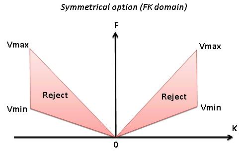
Reject
Option for reject (on) or save (off) data between Vmin and Vmax
• Default: on
• Range: on, off
Taper mode
Type of taper zone between reject and save zones
Min velocity taper
Percent from minimum velocity
•Default: 10 (%)
•Range: from 0 to 100 (%)
Max velocity taper
Percent from max velocity
•Default: 10 (%)
•Range: from 0 to 100 (%)
Wave number taper (Number of K)
Frequency taper
Taper defined by frequency:
• Default: 5 (Hz)
• Range: from 0 to max samplingfrequency (Hz)
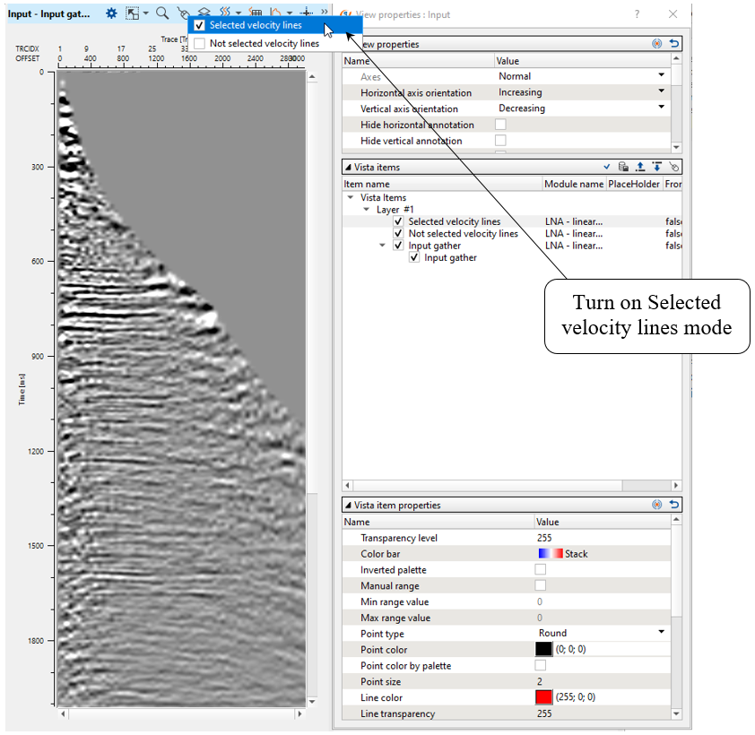
This modules does have interactive velocity range parameter definition. Open all vista groups. Go to the input gather window and activate Selected velocity lines:
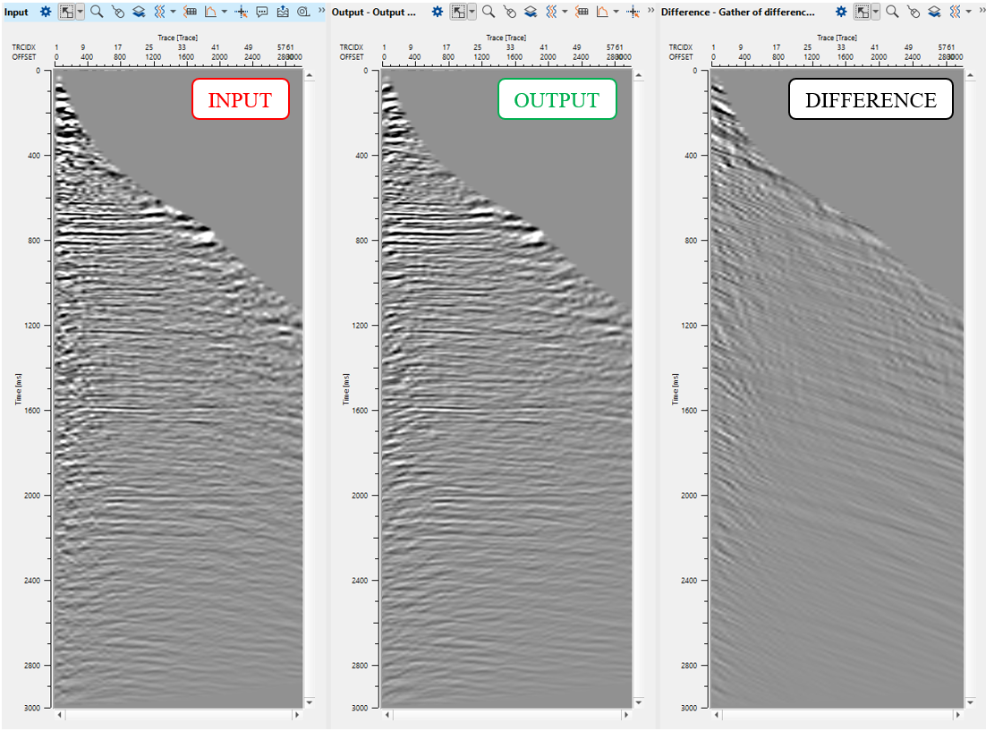
Execute the module, open vista windows and check result:
6) LNA - linear up - We named (commented) this module as linear up, where up means linear wave goes vice versa down-up from zero near to far offset.
Parameters:
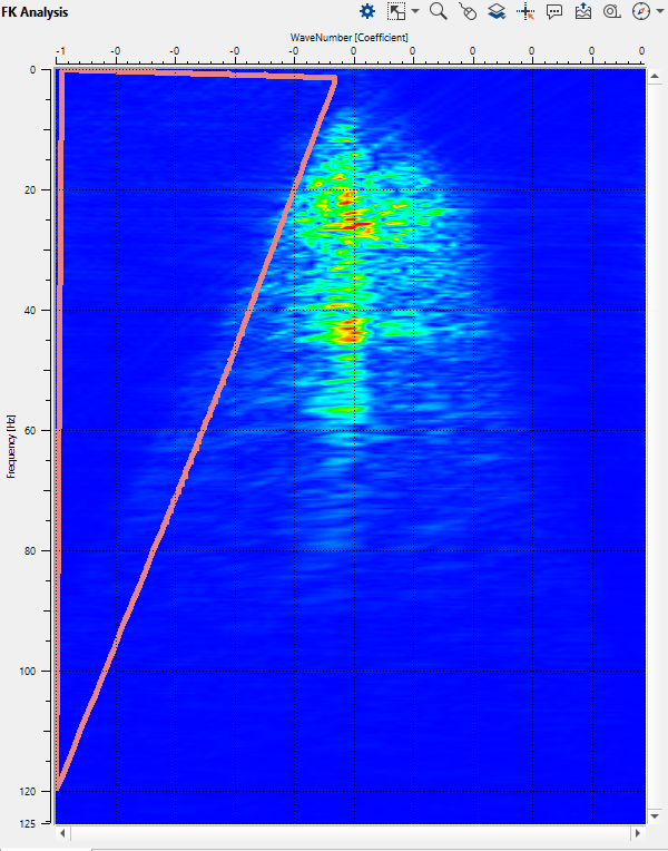
7) FK Filter - linear up - This module applies an FK filter. FK transforms 2D data to frequency-wave number space. A user can then define a mute zone in that space to apply an FK filter. We named (commented) this module as linear up, where up means conventional linear wave, means wave goes vice versa down-up near to far offset. Define parameters:
Parameters:
Open FK Analysis vista window and draw a polygon on the right side of the spectrum:
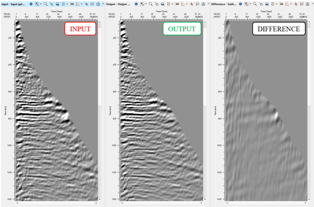
Execute the module and check the result:
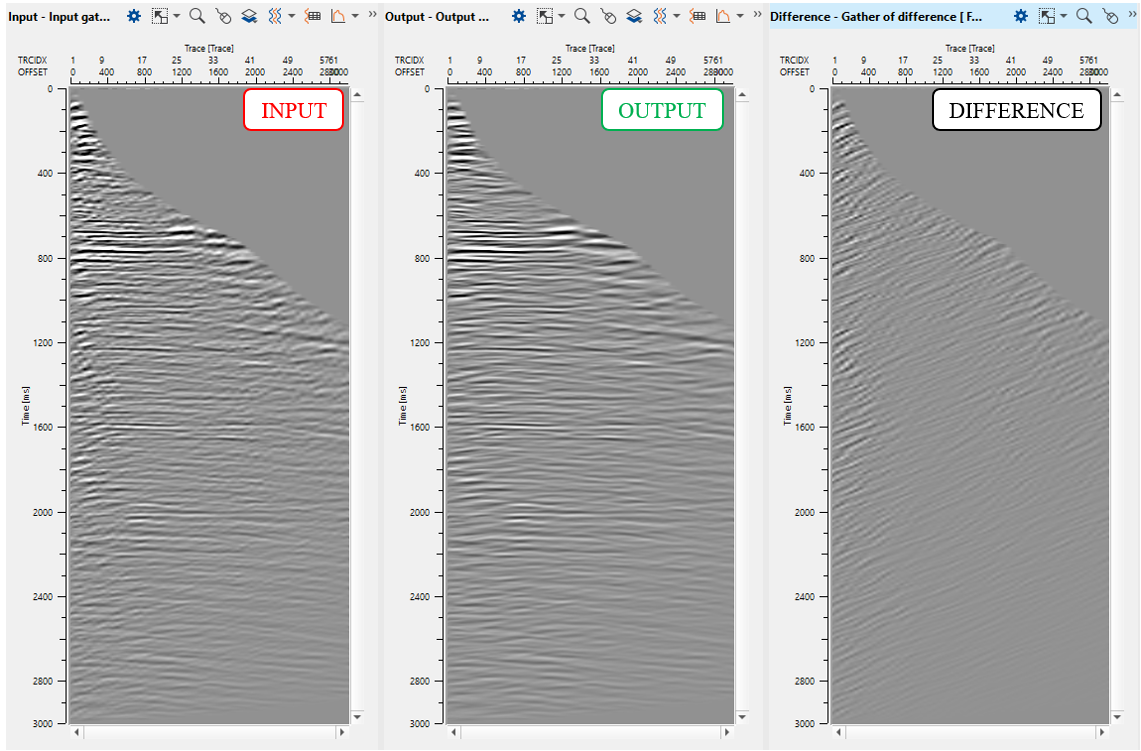
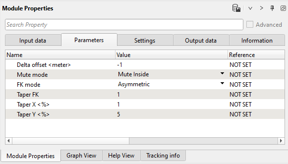
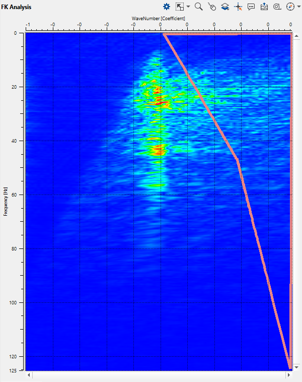
8) FK Filter - linear down - We named (commented) this module as linear down, means conventional linear wave goes up-down from zero near to far offset. Define parameters:
Parameters:
Open FK Analysis vista window and draw a polygon on the left side of the spectrum:
Execute the module and check the result: