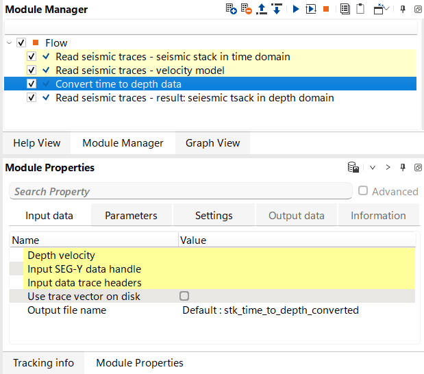
Seismic data conversion from time to depth domain
![]()
![]()
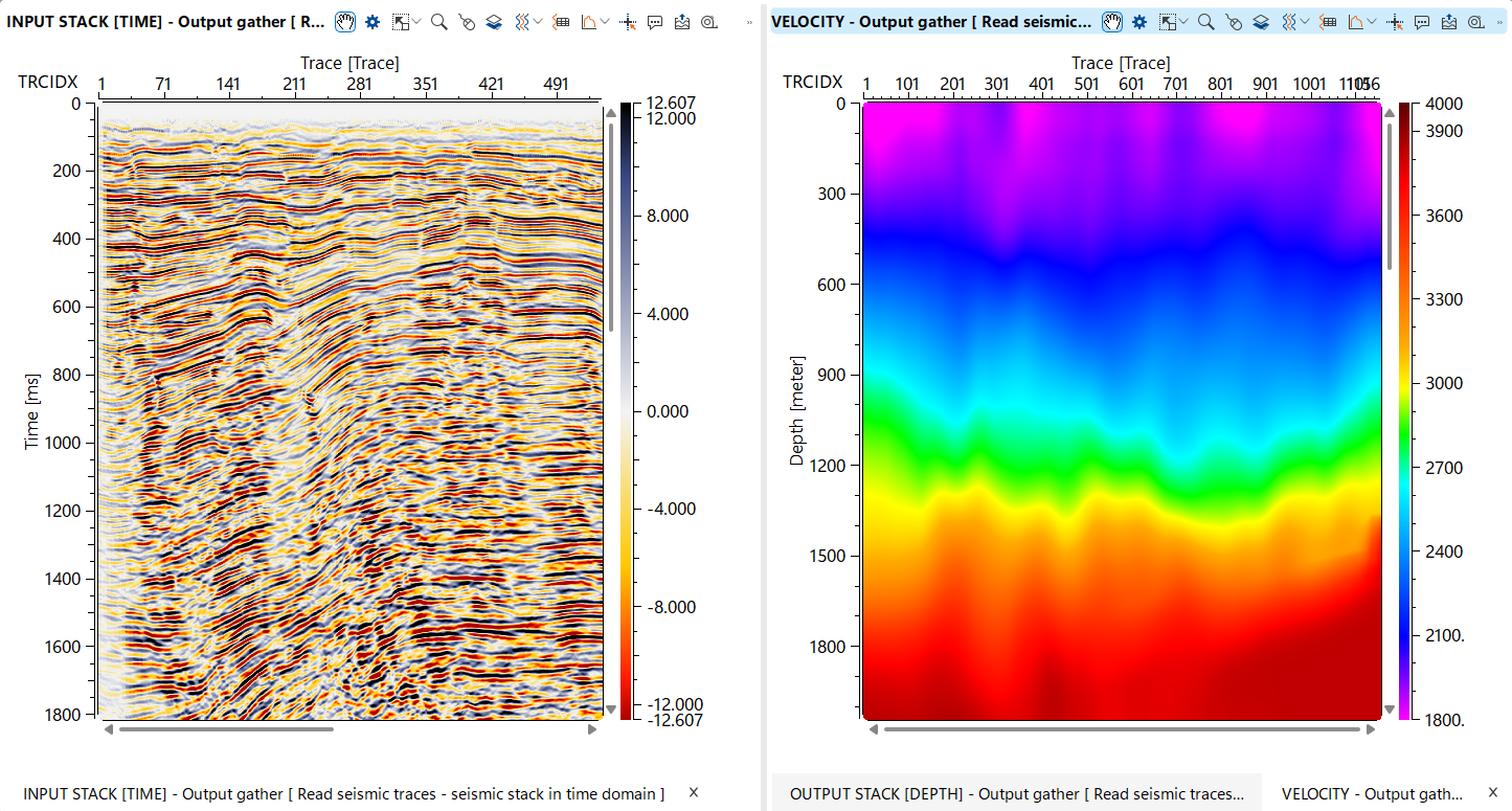
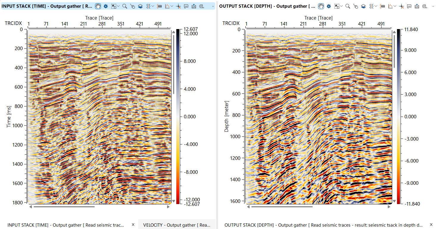
This module converts seismic data from the time domain to the depth domain, a critical step in seismic processing that enables more accurate subsurface imaging and geological interpretation. The module accepts time-domain seismic traces and a depth velocity model describing how seismic wave velocities vary with position and depth. Using this velocity field, it computes one-way travel time tables for each location, optionally smooths them spatially to reduce abrupt lateral velocity changes, and then maps each time sample to its corresponding depth. The output is a depth-domain seismic volume stored in g-Platform native format (.gsd), ready for depth interpretation, attribute analysis, and integration with well data.
![]()
![]()
Depth velocity - depth velocity model that will be used for time to depth conversion. Depth model in gather format in upload to RAM.
Connect the interval velocity gather in the depth domain (typically produced by a velocity model building or depth conversion workflow). The model is loaded entirely into RAM before processing begins, so ensure sufficient memory is available for large 3D velocity cubes. The velocity model must be defined on a constant datum — the module will report an error if source and receiver datums are inconsistent within the model. The spatial coverage of the velocity model determines where accurate depth conversion is possible; traces located outside the model extent will be assigned the nearest available velocity.
Input SEG-Y data handle - link to the seismic data file (usually it is out data set from Read seismic traces module).
This input is active when Use trace vector on disk is set to No. Connect the SEG-Y data handle produced by a Read Seismic Traces module. The module reads the seismic traces from disk in bulk during processing, using the trace header list supplied via the Input data trace headers connection.
Input data trace headers - link to the seismic trace headers (usually it is out data set from Read seismic traces module).
This input is active when Use trace vector on disk is set to No. Connect the trace header vector from the same Read Seismic Traces module as the data handle. The header vector is held in RAM and provides the bin locations and geometry information needed to match each seismic trace to the correct velocity model location.
Use trace vector on disk - there is an extra option for saving RAM in case of very limited computer resources: link to the seismic trace headers on a disk (usually it is out data set from Read seismic traces module). Module will read traces headers directly from disk without necessarily to upload trace header vector into RAM.
When set to Yes (the default), connect the on-disk trace vector item from a Read Seismic Traces module. Trace headers are read directly from disk rather than loaded into RAM, which significantly reduces memory consumption for large datasets. When set to No, use the separate Input SEG-Y data handle and Input data trace headers inputs instead. Use the on-disk mode for very large datasets or when available RAM is limited.
Output file name - define an output file name for resulting seismic data set converted to depth domain.
Specify the full path and file name for the depth-domain output dataset. The file is written in g-Platform native seismic format (.gsd). The output inherits the spatial sampling (inline and crossline intervals) from the input data, while the vertical axis is in depth (m) and the sample interval is determined by the depth velocity model grid spacing. Choose a location with sufficient disk space, as the output volume size is proportional to the number of input traces multiplied by the number of depth samples in the velocity model.
![]()
![]()
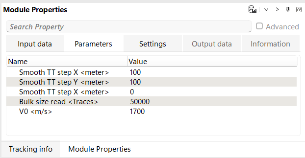
Smooth TT step X - parameter is used to smooth the travel times during the conversion of seismic data from the time domain to the depth domain. It works in conjunction with the velocity model, which provides the necessary information for quickly calculating the travel times of seismic waves. The calculated travel times are then smoothed along the X-axis using this parameter. The smoothing process helps to reduce abrupt changes in travel time, leading to a more accurate and continuous depth conversion.
Sets the spatial smoothing half-window applied to the computed travel time tables in the crossline (X) direction, measured in metres. The default value is 100 m. A value of 0 disables smoothing in this direction. Increasing this value produces smoother lateral variations in the depth conversion, which is useful when the velocity model contains noise or sparse control points. Use smaller values (or zero) when the velocity model is already well-constrained and laterally consistent, to preserve fine structural details.
Smooth TT step Y - parameter is used to smooth the travel times during the conversion of seismic data from the time domain to the depth domain. It works in conjunction with the velocity model, which provides the necessary information for quickly calculating the travel times of seismic waves. The calculated travel times are then smoothed along the Y-axis using this parameter. The smoothing process helps to reduce abrupt changes in travel time, leading to a more accurate and continuous depth conversion.
Sets the spatial smoothing half-window applied to the computed travel time tables in the inline (Y) direction, measured in metres. The default value is 100 m. A value of 0 disables smoothing in this direction. For 2D datasets or when the inline extent is limited, this parameter can be set to zero. In 3D surveys, matching this value to the crossline smoothing window (Smooth TT step X) produces isotropic lateral smoothing of the travel time field.
Smooth TT step Z - parameter is used to smooth the travel times during the conversion of seismic data from the time domain to the depth domain. It works in conjunction with the velocity model, which provides the necessary information for quickly calculating the travel times of seismic waves. The calculated travel times are then vertical smoothed along the Z-axis using this parameter. The smoothing process helps to reduce abrupt changes in travel time, leading to a more accurate and continuous depth conversion.
Sets the vertical smoothing window applied to the computed travel time tables along the depth (Z) axis, measured in metres. The default value is 0 m (no vertical smoothing). Vertical smoothing can reduce high-frequency oscillations in the velocity model that might otherwise cause wavelet stretching or squeezing artefacts in the converted data. Apply this parameter with caution — excessive vertical smoothing may blur thin-layer velocity contrasts that are geologically meaningful.
Bulk size read - portion of the input data for reading from disk.
Controls how many traces are read from disk and processed in each batch. The default value is 50,000 traces. Larger values reduce the number of disk read operations and may improve throughput on fast storage systems, but require more RAM. Reduce this value if the processing machine has limited memory, particularly when working with long traces (many depth samples) or when the velocity model itself is already consuming significant RAM. The minimum value is 1.
V0 - define velocity in he weathering zone (layer).
Specifies the near-surface (weathering zone) velocity used to apply a static shift correction when the input seismic data is not already referenced to topography. The default value is 2300 m/s. The module checks whether each trace is on topography by comparing its source and receiver datum values. If the trace datums differ from the topographic surface elevation, a static correction using this velocity is applied before depth conversion, ensuring that all traces are reduced to the topographic datum before the depth mapping is performed. Set this value to match the average velocity of the near-surface layer in your survey area.
![]()
![]()
SegyReadParams
This group contains SEG-Y reading parameters used when accessing input seismic data via the Input SEG-Y data handle connection (i.e., when Use trace vector on disk is set to No). Configure the byte locations for key trace header fields (inline, crossline, coordinates, etc.) to match the header format of your input SEG-Y file. These settings are only relevant when not using the on-disk trace vector mode.
Execute on { CPU, GPU }
Selects whether the depth conversion computation runs on the CPU or GPU. CPU execution uses multi-threaded processing and is compatible with all systems. GPU execution may offer faster performance on machines equipped with a supported graphics card. Select GPU only if a compatible GPU is available and the dataset is large enough to benefit from GPU acceleration.
Distributed execution
Enables distributed (cluster) processing, allowing the depth conversion to be split across multiple compute nodes. When enabled, the input data is partitioned and each node processes a subset of traces independently. This is recommended for very large 3D datasets where single-node processing would be impractical. Requires a configured g-Platform cluster environment.
Bulk size
Defines the minimum chunk size (in traces) sent to each compute node during distributed execution. Larger chunks reduce inter-node communication overhead but require more memory per node. Adjust this value based on the available RAM per node and the total number of traces in the dataset.
Limit number of threads on nodes
When distributed execution is active, this setting caps the number of CPU threads that each remote node may use. Limiting threads on nodes can prevent resource contention when multiple jobs are running concurrently on shared cluster nodes.
Job suffix
An optional text label appended to the distributed job name. Use this to distinguish between multiple simultaneous depth conversion jobs running on the same cluster, making it easier to identify and monitor individual jobs in the cluster management interface.
Set custom affinity
Enables manual specification of CPU core affinity for the processing threads. When activated, use the Affinity field below to define which CPU cores are used. This is an advanced setting for performance tuning on NUMA or multi-socket systems.
Affinity
Specifies the CPU core mask or list used when Set custom affinity is enabled. Only relevant for advanced cluster or workstation configurations where precise control over CPU resource allocation is required.
Number of threads
Sets the number of parallel CPU threads used for the depth conversion computation. By default, the module uses all available logical cores on the machine. Reducing the thread count frees CPU resources for other processes running concurrently. The depth conversion loop is fully parallelised across traces, so performance scales well with thread count for large datasets.
Skip
When enabled, this module is bypassed entirely and the workflow continues to the next step without performing any depth conversion. Use this option to temporarily disable the conversion during workflow testing or parameter optimisation without removing the module from the processing sequence.
![]()
![]()
![]()
![]()
Workflow example:
![]()
![]()
YouTube video lesson, click here to open [VIDEO IN PROCESS...]
![]()
![]()
 * * * If you have any questions, please send an e-mail to: support@geomage.com * * *