Velocity model tie to wells, Thomsen Delta parameter
![]()
![]()
The Delta Thomsen parameter (Δ) is a key anisotropy coefficient used in seismic velocity modeling to describe anisotropic effects in a transversely isotropic medium (VTI). This parameter accounts for variations in seismic wave propagation due to layered geological structures, where vertical and horizontal velocities differ.
In this module, Δ is derived from the isotropic velocity model tied to well data, enabling a more accurate estimation of subsurface velocity variations. The computed Δ cube is later utilized in the Time Table Calculation module for improved depth conversion and seismic imaging.
Calculation Process in the Module
The module estimates Δ using the following workflow:
1.Input Data & Preprocessing
oAn isotropic velocity model is generated by tying seismic velocities to well log data.
oWells, seismic stacks, and velocity overlays with input and corrected horizons are displayed in interactive windows.
oThe module allows selection of different methods for well surface creation, ensuring an optimal starting point for calculation.
2.Delta Thomsen (Δ) Calculation
oΔ is computed by analyzing the difference between interval vertical velocity (Vint-VTI) and the reference isotropic velocity model.
oThe result is a Delta Thomsen cube, which represents variations in anisotropy throughout the subsurface.
oThis cube is essential for depth conversion, seismic migration, and further anisotropic corrections.
3.Output Products
oVertical Interval Velocity Cube – Represents the vertical velocity variations used for depth modeling.
oDelta Thomsen Cube – Provides anisotropy corrections to enhance seismic imaging accuracy.

![]()
![]()
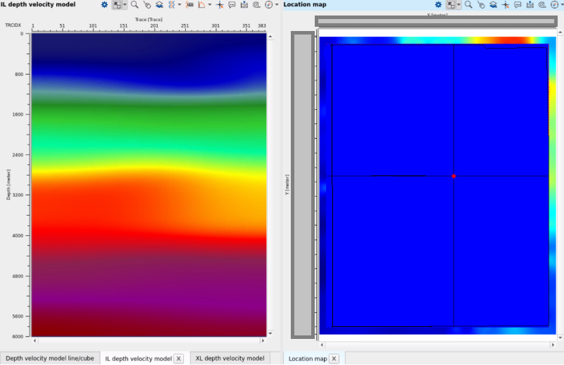
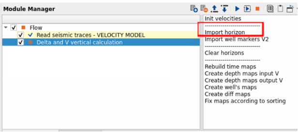
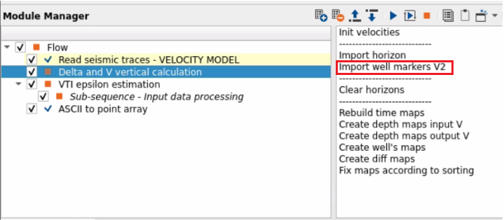
Init velocities - first step in this module is pressing init velocities button for rendering: Location map and Vertical sections.
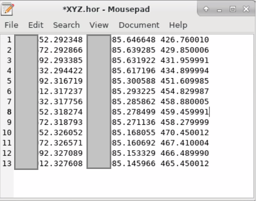
Import horizon - load horizons for tie. Domain is TIME ms! Use separated ASCII files for each horizon and load them individually. This horizon will be automatically interpolated in converted into the depth domain by using input isotropic velocity. File format is ASCII.hor with the following columns (tab-delimited):
Important! Before the import, define its parameters as well, for example datum plane:
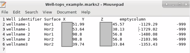
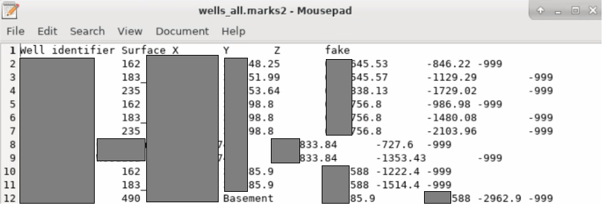
Import well markers V2 - load well tops for tie. Use one single ASCII file for all wells. Well tops in depth m, TVDSS. Pay attention! that module understand the datum plane, because of input velocity file: it reads trace headers RECEIVER_DATUM and SOURCE_DATUM, they are constant values, because this datum was defined during velocity conversion Vrms to Vint. Therefore, if this datum for headers is not 0, module will add datum plane value to well tops (it is for correct tie process). File format is ASCII.marks2 with the following columns (tab-delimited, 1-st row is names of columns, last column must be filled with something like -999):
Clear horizons - remove all horizons form the module.
Rebuild time maps - rebuild time maps in case you changed interpolation parameters for time horizons.
Create depth maps input V - build a horizon map of the input isotropic velocity.
Create depth maps output V - build a horizon map of the output vertical velocity.
Create well's maps - build a horizon map for tie process by using well tops in case you would like to option [Well tie options->Tie type->Strict by wells]. Check this layer in Location map vista after calculation.
Create diff maps - build a difference map between input and output (well-tied) horizons. Check this layer in Location map vista after calculation.
Fix maps according to sorting - use this option in case you would like to import horizons again. When new horizon was imported press fix maps button. All horizons in the module will be sorted by the depth values accordingly.
![]()
![]()
Input gathers - input isotropic velocity (loaded as seismic cube to the workflow).
Input time horizons - input time horizons.
![]()
![]()
V0 <m/s> - replacement velocity in m/s.
Type of creation - where are two types of creation vertical velocity and delta: 1 - smooth and gradient vertical model; 2 - layer vertical model.
Show cube vistas(for 3d) - create a 3D cube for visualization (seismic, velocity, delta, horizons).
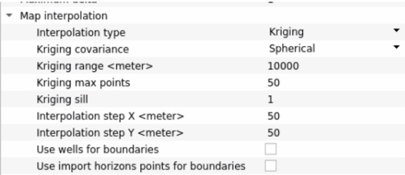
Map interpolation:
Interpolation type - algorithms for map interpolation: Kriging, ABOS.
Kriging covariance - only for Kriging option: Spherical, Gaussian, Exponential.
Kriging range <meter> - only for Kriging option, is a maximum range for getting near point.
Kriging max points - only for Kriging option, is a maximum points for the interpolation.
Kriging sill - is the total variance contribution, or the maximum variability between pairs of points.
Interpolation step X <meter> - step in meters for the interpolation along X axes.
Interpolation step Y <meter> - step in meters for the interpolation along Y axes.
Use wells for boundaries - limit the map bounds by wells.
Use import horizons points for boundaries - limit the map bounds by input horizons.
Well tie options:
Marker distance <meter> - distance for well visualization on the current seismic/velocity stack section. so you can get bigger radius for searching wells around the inline/crossline. Used just for visualization.
Add bottom layer - add bottom layer to the model.
Number of iterations - iteration for tie process. Theoretically, bigger value, more accurate velocity model will be tied to wells.
Minimum velocity <m/s> - minimum velocity in m/s for the output velocity model.
Maximum velocity <m/s> - maximum velocity in m/s for the output velocity model.
Gradient type - there two gradients types for the output velocity model: smooth, simple.
Maximum distance to voronoi interpolation <meter> - distance/radius/area around wells for interpolation.
Maximum extrapolation distance <meter> - distance/radius/area around wells for extrapolation.
Extrapolate deepest layer coeef - explanation...
Allow regression extrapolation - explanation...
Tie type - Strict by wells, Emulate wells, Depth well's maps.
Step type - Grid, Trace.
Emulation step IL - step inline for emulation.
Emulation step XL - step crossline for emulation.
Resample options:
Resample - enable re sample option for velocity model.
Delta z after resample <meter> - depth interval in meters.
Depth maps smooth:
Step X <meter> - smoothing step along X direction.
Step Y <meter> - smoothing step along Y direction.
Smooth depth maps in - enable map smoothing of input horizons in depth.
Smooth depth maps out - enable map smoothing of output horizons in depth.
Smooth depth maps wells - enable map smoothing of wells horizons in depth.
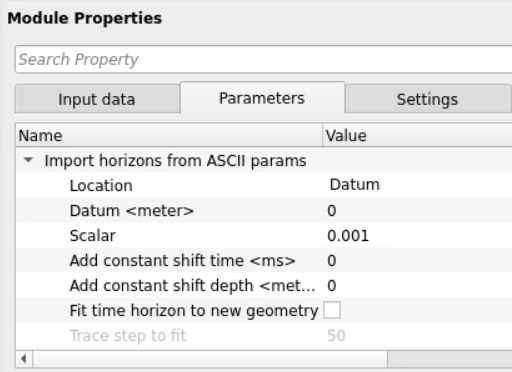
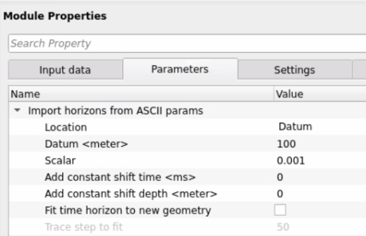
Import horizons from ASCII params:
Location - datum plane for input horizons: Datum is constant value, Topography.
Datum <meter> - value for constant datum plane.
Scalar - explanation...
Add constant shift time <ms> - an additional time shift for input horizons (ms).
Add constant shift depth <meter> - an additional depth shift for input horizons (m).
Fit time horizon to new geometry - explanation...
Trace step to fit - explanation...
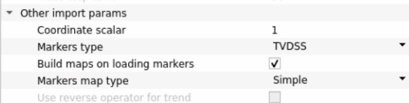
Import marker options:
Coordinate scalar - coefficient for coordinates X, Y.
Markers type - MD (measured depth) or TVDSS (true vertical depth). Use TVDSS.
Build maps on loading markers - enable option for well's map creation on loading.
Markers map type - group of methods for well's map creation: Simple, Trend by depth horizon, Trend2, Trend3
Use reverse operator for trend - for remove
Wells ties:
Well tie params:
Layer name - select the first horizon for tie;
Mark name - select the well top of its (1) horizon;
Trend matrix - explanation...
Const delta for layer option - explanation...
![]()
![]()
Skip - switch-off this module (do not use in the workflow).
Number of threads - perform calculation in the multi-thread mode.
![]()
![]()
Output velocity gather - output vertical velocity model.
Output delta gather - output delta Thomsen parameter.
![]()
![]()
Workflow example:
Load the velocity model using the Read seismic traces module:
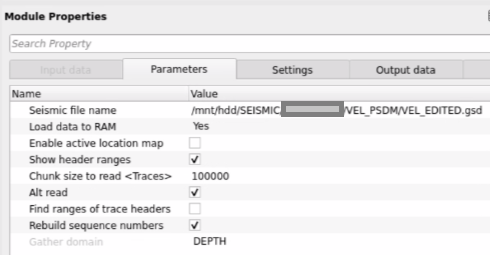
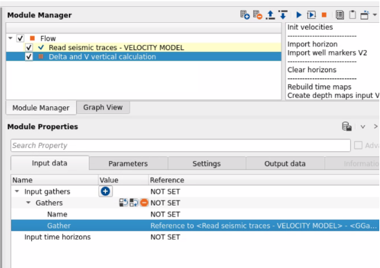
Then we connect this velocity to the Delta and V vertical calculation module:
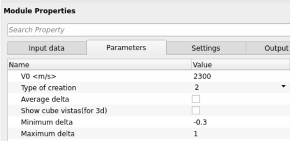
Define replacement velocity:
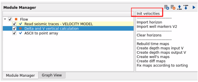
Click the Init velocities button in the action menu to load (initialize) velocities:
Vistas with velocities and map will then be updated, any Inline & Xline on the map can be selected (note that the area boundary polygon on the map is loaded using the ASCII to point array module, and its layer is added to the Location map):
Load horizons in time domain t0, which were picked by the seismic stack cube (in time):
First, in the module parameters we set the datum plane at which the horizon picking was performed, pay attention to the Scalar parameter - it is necessary in order to load a horizon for example from the time domain or the depth domain (if time, then the scalar is 0.001 ms, and if depth, then the scalar is 1)!!!! Change the scalar each time you load different horizons - for example first horizon in time and another time horizon in depth (for example, using your model horizon for tie, i.e. the horizon was prepared separately, e.g. by the interpreter, and we use this horizon for well-tie):
Set Marker type = TVDSS:
Define this group of parameters for gridding, i.e. map creation:
In the action menu click the Import horizon button:
Note the format of the horizons: each horizon is written in a separate ASCII file and looks like this:
X coordinate, Y coordinate, time in ms:
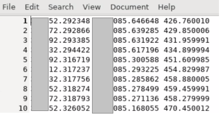
The columns are separated by a tab.
After loading, you can see the horizons in View properties Location map layers and select any one to display:
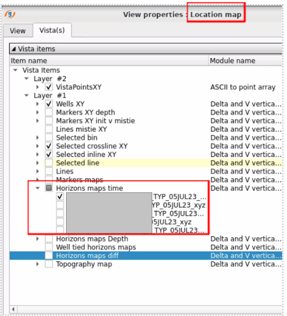
And the map of the selected horizon will be displayed in the Location map window.
Load horizon chops (TVDSS) from borehole data. File format: all chops are recorded in one ASCII file and have the following form:
Well name, horizon name, X coordinate, Y coordinate, depth in m, fake column with any value:
Press on Import well markers V2 in the Action menu:
The markers are then available in the Well XY Location map layer:
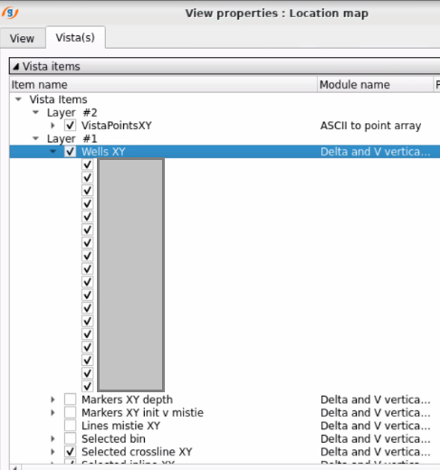
And the loaded wells will be displayed in the Location map window.
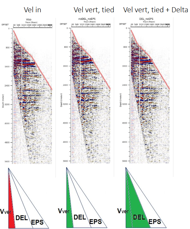
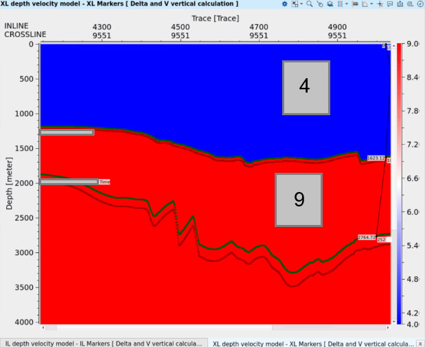
WELL-TIE: The Type of delta creation option = Constant delta
The Type of creation option = Constant delta from well tie params is when we want to enter a constant (average) delta value for each horizon used in the tie, so as not to distort the structural plan of the horizons. Therefore, we will not get the minimum tie values, but they will decrease with respect to the original tie values. This method was used on the project because of uncertainty in the correlation of the horizons, and uncertainty in the quality of the borehole bounces.
Parameters for constant delta:
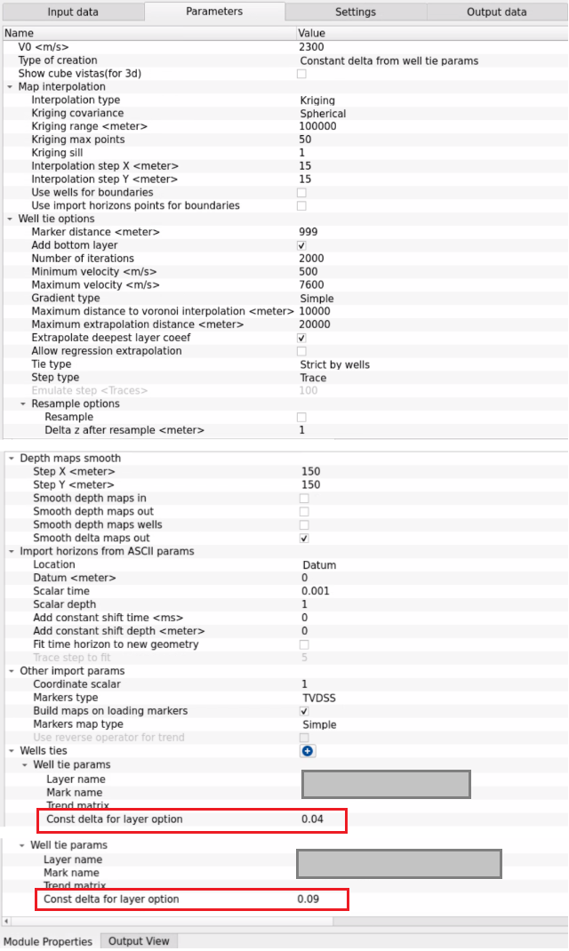
The value of Const delta for layer option is taken from the module's incoherence table, column Delta int before %, for the first horizon:
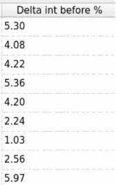
Here the average value is 4, so we specified 0.04 (4/100) in the parameters. Also for the second horizon, the value is 9, divided by 100, we get the parameter 0.09. Example of vertical delta cut for two horizons:
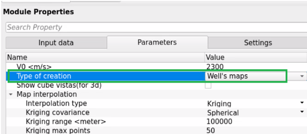
WELL-TIE: The Type of delta creation option = Well's map
The option of linkage method Type of creation = Well's map is when we want to perform linkage using the horizon map built on the basis of wells + trend on the input horizon or performing linkage on the loaded model horizon (e.g. prepared by the interpreter (verb Import well horizon)):
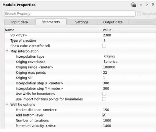
Final parameters for tie:

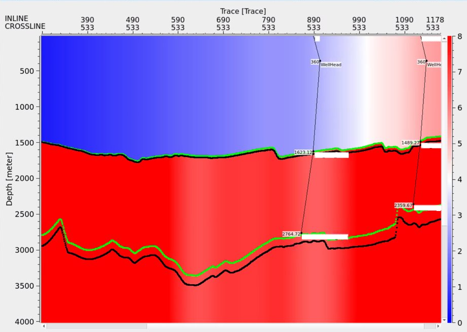
Calculated Delta vertical section with well tops:
![]()
![]()
YouTube video lesson, click here to open [VIDEO IN PROCESS...]
![]()
![]()
 If you have any questions, please send an e-mail to: support@geomage.com
Parameters
The following sections describe all parameters available in the Delta and V vertical calculation module. Parameters are organized into groups that correspond to the collapsible containers visible in the module panel.
Input gathers
A repeatable collection of named input velocity gathers. Each entry consists of a Name label and a connected velocity gather (displayed as a depth-domain trace panel). Connect one or more input velocity models here — typically the interval or RMS velocity field that you want to tie to well control. Multiple gathers can be added to process several velocity models simultaneously, each producing a corresponding output pair (vertical V and Delta).
Input time horizons
A seismic horizon picking item containing the time-domain horizons that define layer boundaries. These horizons are used to compute layer-by-layer depth maps and to constrain the well-tie interpolation spatially. The module converts the time horizons to depth using the input velocity and then matches them against well marker depths to derive the Thomsen delta (Δ) field for each layer. Import horizons from ASCII files using the Import horizon action, or connect them directly from a horizon picking item already in the project.
V0 (replacement velocity)
The reference (replacement) velocity used for the near-surface or above-datum layer, in m/s. Default: 1500 m/s. This value is applied in the uppermost layer (above the first horizon) where no well control is available. For marine surveys, 1500 m/s (water velocity) is appropriate. For land surveys, set this to the near-surface replacement velocity used in your statics workflow.
Type of creation
Selects the method used to compute the Thomsen Delta (Δ) parameter and the vertical velocity (V vertical) field. Default: Well's maps. Six options are available:
Well's maps — The default and most commonly used mode. Well marker depths are loaded and interpolated spatially to build layer-by-layer depth maps. The module then derives per-layer delta values by comparing the time-depth relationship at well locations against the seismic velocity model. This mode provides a fully spatially variable delta field and is the recommended choice when sufficient well control is available.
Constant delta from well tie params — Applies a single delta value per layer as specified in the Well tie params collection. Use this mode when you have only a few wells or want to apply a geologically guided constant anisotropy assumption per layer. In this mode the Average delta, Minimum delta, and Maximum delta controls become active.
Create simple delta — Computes delta by directly matching the time-to-depth conversion at each well location, without applying a thickness trend correction. Suitable for areas with relatively flat or slowly varying anisotropy.
Create delta using thickness trend — Extends the simple delta method by incorporating a spatial trend derived from layer thickness variations. This mode improves delta estimation in areas where anisotropy correlates with structural relief or compaction-driven thickness changes.
Create delta via depth velocities — Derives the delta field by using the depth-domain interval velocity model directly. The module applies a well-tie filter (iterative least-squares optimization, controlled by the Well tie options parameters) to match predicted depths to measured well marker depths. Use this mode when you have a well-conditioned interval velocity model in depth.
Vertical velocities — An alternative well-tie approach that derives the true vertical-propagation velocity (V0, zero-offset velocity) directly from the well data. Use this mode when your goal is to produce a vertical velocity model rather than an explicit delta field.
Average delta
When enabled, the delta values derived from individual wells are averaged across the survey area before being applied, instead of being interpolated spatially. Default: disabled. This option is only active in Constant delta from well tie params mode. Enable it when you want a single representative delta value that reflects the average anisotropy of the whole survey, rather than applying spatial variation.
Minimum delta
The lower clipping threshold applied to the computed delta field. Default: -0.3. Only active in Constant delta from well tie params mode. The Thomsen Delta parameter is dimensionless; physically realistic values for most sedimentary rocks lie in the range -0.1 to 0.3. Setting a minimum prevents spurious negative anisotropy in poorly constrained areas.
Maximum delta
The upper clipping threshold applied to the computed delta field. Default: 1.0. Only active in Constant delta from well tie params mode. Lower this value to prevent unrealistically large anisotropy corrections in areas far from well control.
Show cube vistas (for 3D)
When enabled, the inline and crossline velocity and delta gathers are displayed as full 3D cube panels in the vista windows. Default: disabled. Enable this option when working on 3D surveys and you want to visually inspect the velocity and delta volumes along arbitrary inline and crossline slices. Enabling this may increase display update time for large 3D datasets.
Map interpolation
These parameters control how horizon depth maps are built from the well marker and horizon point data. The resulting maps define the spatial distribution of delta and vertical velocity across the survey area.
Interpolation type
The spatial interpolation algorithm used to build the delta and depth maps from scattered well and horizon control points. Default: ABOS. Two options are available: ABOS (Adaptive B-spline operator — a fast least-squares fitting method well suited to dense, regularly sampled horizon grids) and Kriging (a geostatistical method that accounts for the spatial correlation structure of the data). Use Kriging when your control points are sparse and unevenly distributed, or when you want to honour a specific variogram model.
Kriging covariance
The variogram model used by the Kriging interpolator to describe how the spatial correlation of delta values decreases with distance. Default: Spherical. Options are Spherical (reaches zero correlation at the range distance — good for data with a clear correlation length), Gaussian (smooth, gradual decorrelation — best for smoothly varying fields), and Exponential (faster initial decorrelation — suited to more erratic spatial variation). Only active when Interpolation type = Kriging.
Kriging range
The spatial correlation range of the Kriging variogram model, in metres. Default: 100000 m. Points separated by a distance greater than the range are treated as spatially uncorrelated. Set this to approximately the typical spacing between wells or the geologically expected scale of lateral anisotropy variation. Only active when Interpolation type = Kriging.
Kriging max points
The maximum number of neighbouring control points used in each Kriging estimation. Default: 50. Limiting the neighbourhood improves computation speed. Increase this value when you have dense well coverage and want the interpolated map to honour more nearby data points simultaneously. Only active when Interpolation type = Kriging.
Kriging sill
The sill of the Kriging variogram, representing the total variance of the spatial data. Default: 1.0. This parameter scales the covariance model. In most workflows the default value of 1 is sufficient. Only active when Interpolation type = Kriging.
Interpolation step X / Interpolation step Y
The output map grid cell size in the X (inline) and Y (crossline) directions, in metres. Default: 50 m each. This determines the resolution of the interpolated depth and delta maps. Use a step size comparable to the seismic bin spacing for compatibility with the velocity gather grid. Coarser steps speed up map construction but may miss sharp lateral velocity contrasts between wells.
Use wells for boundaries
When enabled, the convex hull of the loaded well locations is used to define the boundary of the interpolated maps, restricting the output to the area of well coverage. Default: disabled. Enable this option to prevent extrapolation of the delta model into areas with no well control, which can introduce unreliable anisotropy values.
Well tie options
These parameters control the iterative well-tie optimization process that adjusts the velocity model at each well location so that the synthetic time-depth curve matches the measured well marker depths. They are primarily relevant for the Create delta via depth velocities and Vertical velocities creation modes.
Marker distance
The maximum lateral search radius, in metres, within which velocity traces are considered when computing the well-tie at a given well location. Default: 150 m. Increase this value if wells are located between CDP bins and you want to use more surrounding traces to stabilize the tie. Decrease it for high-density surveys where only the nearest traces should contribute.
Add bottom layer
When enabled, the module automatically appends a synthetic bottom layer below the deepest horizon, extending the velocity and delta model to the full record length. Default: enabled. Keep this enabled to avoid gaps in the output velocity model below the last well-constrained horizon.
Number of iterations
The number of iterations in the iterative least-squares well-tie optimization. Default: 2000 (range: 10 to 100000). Higher iteration counts improve convergence accuracy at the cost of longer computation time. Increase this value if the well-tie residuals (mis-tie table) remain large after running with the default. The default of 2000 is adequate for most surveys.
Minimum velocity
The lower bound on the adjusted vertical velocity produced by the well-tie solver, in m/s. Default: 1550 m/s. This prevents the optimizer from producing physically impossible sub-water velocities. For land surveys, you may raise this to the local near-surface velocity.
Maximum velocity
The upper bound on the adjusted vertical velocity, in m/s. Default: 7600 m/s. This prevents the solver from producing unrealistically high velocities in poorly constrained areas. Reduce this value if your target formations are known to have velocities well below this limit.
Gradient type
Controls the gradient descent strategy used in the iterative well-tie optimization. Default: Simple. Simple uses a standard steepest-descent step and converges quickly for well-conditioned problems. Smooth applies additional regularization to the gradient, which can improve stability in areas with sparse well control or noisy velocity functions.
Maximum distance to voronoi interpolation
The maximum distance, in metres, over which the well-tie correction is spread using Voronoi (nearest-neighbour) spatial interpolation between wells. Default: 10000 m. Grid points located further than this distance from the nearest well are handled by extrapolation instead. Increase this value to extend the well-tie influence over a larger area.
Maximum extrapolation distance
The maximum distance from the outermost well, in metres, beyond which the module will not extrapolate the well-tie correction. Default: 20000 m. Beyond this limit the velocity model is left unmodified. Set this to zero to disable all extrapolation and restrict the output strictly to the area bounded by wells.
Extrapolate deepest layer coefficient
When enabled, the well-tie correction coefficient derived for the deepest constrained layer is applied to all deeper (unconstrained) samples below it. Default: enabled. This ensures that the output velocity model has a smooth, geologically consistent continuation below the deepest well marker, rather than reverting to uncorrected seismic velocities.
Allow regression extrapolation
When enabled, a regression-based (trend) extrapolation is used beyond the maximum extrapolation distance, rather than leaving the model unchanged. Default: disabled. Enable this only when the survey area extends far beyond the well coverage and you want a geologically guided continuation of the delta trend into undrilled areas.
Tie type
Determines how the well-tie correction is applied across the survey. Default: Strict by wells. Strict by wells — The optimization is driven exclusively by the loaded well marker depths; all correction is anchored to real well data. Emulate wells — Pseudo-well locations are generated at a regular grid spacing across the survey and used to stabilize the interpolation in areas without real well coverage. This is useful for surveys with only one or two real wells.
Step type / Emulate step
When Tie type = Emulate wells, these parameters define the spacing of the pseudo-well grid. Step type selects whether the spacing is in trace units (Trace, default) or by inline/crossline grid indices (Grid). Emulate step sets the spacing in traces (default: 100). Emulate step IL and Emulate step XL set the inline and crossline grid spacing respectively (default: 10 each). A finer emulated grid provides smoother interpolation between real wells but increases computation time.
Resample options
Controls depth resampling of the output velocity and delta gathers. Resample: enabled by default. When enabled, the output is resampled to a uniform depth step defined by Delta z after resample (default: 1 m). A uniform 1 m depth step is standard for most depth-domain velocity models and ensures compatibility with depth migration workflows. Disable resampling only if you need to preserve the original irregular depth sampling of the input gathers.
Depth maps smooth
These parameters apply a spatial smoothing filter to the intermediate and output depth maps before they are used for well-tie interpolation and delta computation. Smoothing suppresses noise from irregular well distributions or sparse horizon picks.
Step X / Step Y
The smoothing radius in the X (inline) and Y (crossline) directions, in metres. Default: 150 m each. Larger values produce smoother maps and suppress short-wavelength noise, at the expense of spatial resolution. Set this to approximately one to two CDP spacings for standard surveys. For surveys with dense, reliable horizon picks this can be set smaller, or smoothing can be disabled by unchecking the individual smooth toggles below.
Smooth depth maps in
When enabled, smoothing is applied to the input depth maps (derived from the input time horizons and the seismic velocity). Default: enabled. Smoothing the input depth maps helps suppress noise in the seismic velocities before the well-tie optimization is applied.
Smooth depth maps out
When enabled, smoothing is applied to the output depth maps (derived from the well-tied vertical velocity). Default: enabled. This produces geologically consistent, smoothly varying output depth horizons suitable for use as structural constraints in depth migration.
Smooth depth maps wells
When enabled, smoothing is applied to the depth maps built from well marker positions before they are used in the interpolation. Default: enabled. This avoids sharp discontinuities in areas with isolated wells that deviate from the regional structural trend.
Smooth delta maps out
When enabled, smoothing is applied to the output Thomsen Delta (Δ) maps before they are used to build the output delta gather. Default: enabled. Smoothed delta maps reduce artefacts from sparse well control and produce a more stable anisotropy model for depth migration.
Import horizons from ASCII params
These parameters configure the loading of time horizons from external ASCII text files, triggered by the Import horizon action. The expected file format is tab-separated columns: X coordinate, Y coordinate, two-way time (in ms, scaled by Scalar time).
Location
Defines the vertical reference surface from which horizon times are measured. Default: Datum. Datum — horizons are referenced to the flat datum elevation specified by the Datum parameter. Topography — horizons are referenced to the topographic surface. Use Topography for land surveys with significant surface relief where the datum and the topography differ substantially.
Datum
The datum elevation, in metres, used as the reference surface when Location = Datum. Default: 0 m. Set this to the seismic datum elevation used during processing. For offshore surveys the datum is typically the sea surface (0 m).
Scalar time
A multiplier applied to the time values read from the ASCII horizon file to convert them to seconds. Default: 0.001 (converts milliseconds to seconds). If your ASCII file already stores times in seconds, set this to 1. If the file stores times in another unit, adjust the scalar accordingly.
Scalar depth
A multiplier applied to depth values read from the ASCII file. Default: 1 (no conversion; depths assumed to be in metres). Set to 0.3048 if the file stores depths in feet.
Add constant shift time / Add constant shift depth
A constant time offset (in seconds) or depth offset (in metres) added to all horizon samples after loading. Default: 0 for both. Use these to apply a bulk static shift to imported horizons when there is a known systematic offset between the horizon file and the seismic data — for example, to correct for a datum difference between the horizon interpretation and the seismic processing datum.
Fit time horizon to new geometry
When enabled, the imported horizon is re-interpolated onto the CDP geometry of the connected velocity gathers using the step defined by Trace step to fit. Default: disabled. Enable this when the imported horizon has a different spatial sampling from the velocity gather grid, to ensure a consistent bin-by-bin match.
Trace step to fit
The trace decimation step used when fitting the imported horizon to the velocity gather geometry. Default: 5. Only active when Fit time horizon to new geometry is enabled. A larger step makes the fitting faster but less accurate for steeply dipping horizons.
Import markers options
These parameters configure the loading of well marker (well top) depth data from external ASCII files, triggered by the Import well markers V2 action. Well markers define the measured or true-vertical subsea depths of formation tops that anchor the delta computation to real borehole data.
Coordinate scalar
A multiplier applied to the XY coordinates read from the well marker file. Default: 1 (no scaling). Use this if the coordinate system in the marker file differs from the project coordinates by a constant scale factor — for example, to convert from kilometre to metre units.
Markers type
Specifies the depth convention used for the marker depths in the import file. Default: MD (measured depth). MD — depths along the borehole path (for deviated wells a deviation survey is used for conversion to vertical depth). TVDSS — true vertical depth below the reference surface (sea level or datum). Use TVDSS for pre-converted marker files; this is the most common choice for offshore projects.
Build maps on loading markers
When enabled, the well marker maps (showing well positions and depths in the location map) are rebuilt automatically as soon as markers are imported, without requiring a separate Create well's maps action. Default: enabled. Disable this if importing a large number of markers and you want to defer map building to a later step.
Markers map type
Controls the spatial interpolation trend applied when building well marker depth maps from discrete well locations. Default: Simple. Simple — direct interpolation of well marker depths with no structural guide. Trend by depth horizon — uses the shape of the corresponding depth horizon as a structural guide, preserving the relative depth relationship between wells. Trend by time horizon — uses the time-domain horizon shape as the structural guide. The Trend options produce geologically more realistic marker maps in structurally complex areas.
Use reverse operator for trend
When enabled and a trend-based marker map type is selected, the structural trend is applied using the inverse of the trend operator. Default: disabled. Use this option when the horizon structural dip produces an over-corrected marker map, and inverting the trend operator brings the result closer to the observed well depths.
Well tie params
A repeatable collection that assigns a per-layer delta value when using the Constant delta from well tie params creation mode. Each row corresponds to one stratigraphic layer, identified by its layer name and associated well marker name. Add one row per layer (per horizon interval) that you want to assign a specific constant delta value.
Layer name
The name of the horizon layer (depth interval) to which this constant delta entry applies. The dropdown is populated from the imported horizons. Select the layer whose top boundary you want to assign a delta value.
Mark name
The well marker name associated with this layer. The dropdown is populated from the imported well markers. This links the chosen layer to the well formation top used to calibrate the delta value for that interval.
Const delta for layer option
The constant Thomsen Delta (Δ) value applied uniformly across the survey for this layer. Default: 0 (isotropic — no anisotropy correction). Positive delta values indicate that the NMO velocity is greater than the true vertical velocity, which is typical for shales and compacted sediments. Set each layer's value based on well analysis or published analogue data for the local geology.
Output data
The module produces the following output items after execution.
V vertical (output collection)
A collection of named depth-domain velocity gathers containing the well-tied vertical (zero-offset) P-wave velocity model. Each output gather corresponds to one of the input velocity gathers and carries the same name. Connect this output to depth migration modules that require a vertical velocity field to correctly account for VTI anisotropy in depth imaging.
Delta vertical (output collection)
A collection of named depth-domain gathers containing the Thomsen Delta (Δ) anisotropy parameter, sampled on the same depth grid as the vertical velocity output. Each trace represents the spatial distribution of delta at a given CDP location. Connect this output to VTI depth migration modules as the delta input that controls the ray-bending correction due to anisotropy. Inspect these gathers in the Output delta vista to verify that derived delta values are geologically plausible before migration.
Output time horizons
The horizon picking item containing the time horizons after any geometry-fitting or resampling applied during the import workflow. This output can be passed to downstream modules that require horizon data, such as layer-based tomography or depth conversion modules.
Mis tie table
A quality-control table listing the residual depth difference (mis-tie) at each well location, for each marker, after the well-tie optimization. Review this table after execution to identify wells where the depth prediction is poor. Large mis-ties indicate either incorrect marker depths, a velocity model inconsistent with the well data, or insufficient optimization iterations. Use this information to guide further QC and parameter adjustment before finalizing the anisotropy model.
Actions
The following actions are available in the module action menu. They control data import and intermediate map construction steps and should generally be run in the order listed for a standard workflow.
Init velocities
Loads and initializes the input velocity gathers from the connected input data items. Run this action first after connecting the input velocity models, before importing horizons or markers. This populates the velocity display vistas (Input V, Output V, Output delta) so that you can verify the data is correctly loaded.
Import horizon
Opens a file browser to select an ASCII horizon file for import. The file must contain tab-separated columns: X coordinate, Y coordinate, two-way time (in ms, scaled by Scalar time). Multiple horizons can be imported sequentially; each is stored as a separate layer. After import, the horizon appears in the Horizons depth layer of the vista display.
Import well markers V2
Opens a file browser to import well marker (well top) data from an ASCII file. The depth convention is set by the Markers type parameter (MD or TVDSS). Loaded well markers are shown in the Wells XY and Markers XY depth location map layers. If Build maps on loading markers is enabled, the well marker maps are rebuilt automatically after import.
Import well horizon
Imports depth-domain horizon data directly from well logs or existing depth horizon files. Use this action to import horizons that are already in depth (rather than time), bypassing the time-to-depth conversion step for those layers.
Clear horizons
Removes all currently loaded horizons from the module, allowing you to start the horizon import process from scratch. Use this action when you need to replace incorrectly imported horizons or to reset the module state for a new dataset.
Rebuild time maps
Rebuilds the time horizon maps from the currently loaded horizon data. Run this action after modifying horizon import parameters or after adding new horizons, to update the map display without re-running the full module execution.
Create depth maps input V
Converts the loaded time horizons to depth using the input velocity model and builds the input depth maps. These maps represent the predicted depth of each horizon according to the seismic velocity, before any well-tie correction. Review them in the Horizon depth maps vista to assess the structural fit of the velocity model to the well data.
Create depth maps output V
Builds the output depth maps using the well-tied vertical velocity model. These maps show the predicted depth of each horizon after the anisotropy correction has been applied, and should match the well marker depths closely. Compare these maps against the input depth maps to assess the magnitude and spatial pattern of the well-tie correction.
Create well's maps
Builds the well marker depth maps by spatially interpolating the loaded well marker depths across the survey area using the settings in the Map interpolation group. Run this action after importing well markers, or whenever interpolation parameters have been changed, to update the well map display. These maps are the spatial reference used by the well-tie optimization.
Create diff maps
Computes and displays the difference (residual) maps between the input depth maps and the well marker depth maps, and between the output depth maps and the well marker depth maps. Use these maps to identify areas of large depth mis-tie that may require attention before finalizing the anisotropy model.
Fix maps according to sorting
Applies a consistency check and correction to the depth maps to ensure that horizon depths are monotonically increasing with layer index (no depth reversals between layers). Run this action if the mis-tie maps show horizon crossings or anomalous depth inversions that are not geologically expected.