High resolution multiple attenuation in the Radon domain
![]()
![]()
Conventional Radon demultiple algorithm has less quality in case of limitation in small moveout between primaries and multiples (near offsets), as well as when seismic data is aliased. Therefore, those limitats can be overcome by an upgrading of the usual Radon algorithm by enhancing the focusing of energy in the Tau-P domain. The result has better separation of primaries and multiples and better resistance to errors because of different types noise and aliasing.
In other words, High Resolution (HR) Radon module consist of two steps: Radon transform and enhance (focusing) events in Tau-P domain. The main basis is the same as Radon-TauP module has, i.e. this module transforms seismic traces into Tau/P (intercept time and slowness dt/dx = p) domain where we can easily separate multiples and primaries. Such separation allows to attenuate energy of multiple waves before reverse transformation into time domain (T-X). Basic idea is separation primaries and multiples by their velocity (moveout). Input traces are decomposed so hyperbolic events map to elliptical curves in Tau-P domain.
Input seismic gather must be sorted by Common Middle Point (CMP) - Offsets and the primaries should be flattened by applying Normal Move Out (stack velocity) correction before Radon transform. In this case the primary energy will be near P=0, which produces difference in moveout makes it possible to flatten the primary reflections while leaving the multiples under-corrected with a moveout approximately parabolic (Fig.1).
Slowness = 1 / Velocity
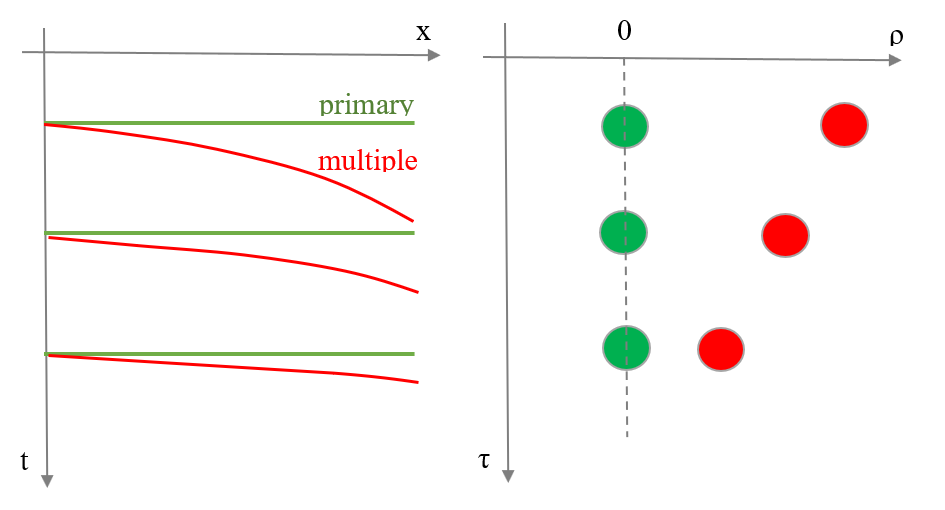
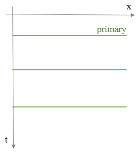
Figure 1. Model of CMP gather: 1) Time domain (T-X): Primaries+Multiples;
2) Tap-P domain: Primaries+Multiples:
3) Time domain (T-X): Primaries.
The module performs a model of primary and multiple events. This computation is based on data decomposition into user-defined parabolas and calculated by high-resolution algorithm, de-aliased least-squares method in the frequency space domain for every frequency of the pass-band which is defined by frequency min (Hz) and frequency max (Hz) parameters. Events corresponding to parabolas with a bigger curvature are considered as multiples. Events corresponding to parabolas smaller than this constrain are primary events. The area limits between primaries and multiples is user defined parametrization.
To avoid drawbacks of conventional Radon transform there was developed upgraded one decomposition is the HR Radon transform. HR Radon method does not have such limitations like conventional algorithm by constraining the parabolic decomposition of the data. These constrain the Radon spectra to be sparse in q and t, using a re-weighted iterative approach. It performs a sparse decomposition of the input seismic data and as result there are less events in the Radon domain, i.e. we have less artifacts due to the smoothing effect in Tau-P domain (Fig.2). The constraints have the effect of moving energy towards those locations where the standard transform has its larger amplitudes, which are predominantly where the energy would sit if there were no sampling or aperture limitations in the input data or in the transform itself. The high-resolution transform is capable, therefore, of better discriminating between primary and multiples and is also resistant to spatial aliasing of the input data.
Conventional Radon HR Radon
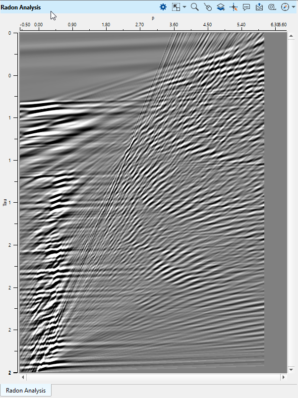

Figure 2. Tau-P transform, compare conventional (left) and high resolution (right).
However, such an iterative approach presents the major drawback of being very much time and computer consuming, so you need to pay more attention to the iteration parameter.
![]()
![]()
No actions
![]()
![]()
Gather - NMO corrected, CMP-Offset sorted.
![]()
![]()
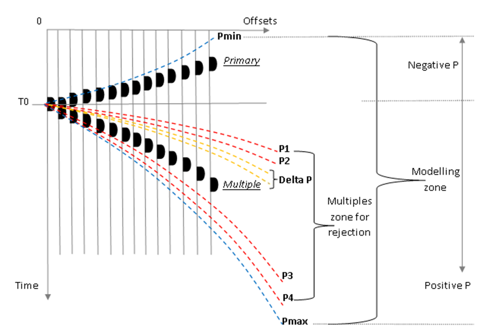
Figure 3. NMO-corrected (intermediate velocity) CMP gathers with main parameters. Note! primary reflection has over-correction for better separation from multiples, but it is not necessary to use special intermediate velocities over-correct hodograph. Also you can apply the final velocity to the CMP gathers for flattening primary reflection.
Minimum p-value for transform data from t-x into tau-p domain.
Enter the minimum p-value of interest, in ms. This value represents the largest over correction on the data at the far offset. Start with a value around -300 ms. Allow the primaries to show a slight over correction.
Maximum p-value for transform data from t-x into tau-p domain. (Choose this parameter with care because run time for this process increases with the square of the number of P-values).
Put the maximum p-value of interest, in ms. Parameter represents the largest under correction on the input data at the far offset. Begin with a value of around 1000 ms. It depends on the data, the velocities of the multiple energy, and the maximum offsets on the input data set.
Increment between parabolas at offset reference offset. This parameter controls the number of functions that are built and the computation time. An value of 20 to 32 ms is usually sufficient, should be approximately equal the signal response time interval.
Parameter for reject or save P taper zones.
Reference offset for modeling. Big value of residual moveout is usually common for far offsets. The reference offset should be close to the maximum offset of the input data.
P zone inside P min/max - values for saving or rejecting:
P1 - Start saving/rejecting zone.
P2 - Taper zone between P1-P2.
P3 - Taper zone between P3-P4.
P4 - End saving/rejecting zone.
Tau taper zone of trace (data):
Tau 1 - Start saving/rejecting zone.
Tau 2 - Taper zone between P1-P2.
Tau 3 - Taper zone between P3-P4.
Tau 4 - End saving/rejecting zone
There are two parameters for solver HR Radon:
Number of iteration - defines the number of iterations for performing the solution iteratively; number of iteration for enhance/focusing events in Tau-P domain.
Tolerance % - threshold for filtering events in Tau-P domain, i.e. bigger value - sparser solution.
Ignore sorting of the input gather - input data set may have any sorting.
Time window - size of the time-sliding window.
Pre-Whitening Factor
Pre-whitening factor (%) for stabilizing tau-p – t-x transformation.
Input traces go though the equalization process before processing and reverse equalization after processing.
Length of the equalization operator.
Parabolic - parabolic transform algorithm.
Foster-Mosher hyperbolic - Foster-Mosher transform algorithm.
Linear tau-p - linear transform algorithm is usually used for linear de-noise task.
Abs linear tau-p - abs linear transform algorithm is usually used for linear de-noise task.
Split to positive/negative offsets - separate data into negative and positive offsets.
![]()
![]()
Skip - switch-off this module (do not use in the workflow).
Auto-connection - module is connected with previous (and next) modules in the workflow by default.
Bad data values option
There are 3 options for corrupted (NaN) samples in trace:
Fix - fix corrupted samples.
Notify - notify and stop calculations.
Continue - continue calculations without fixing.
Calculate difference - display gather difference (DIFF = IN - OUT). By default difference is empty.
![]()
![]()
Gather - NMO corrected, CMP-Offset sorted.
![]()
![]()
A test seismic data set is Viking Graben 2D (marine), you can download it using the following link Dataset.sgy
An example of the workflow for demultiples:
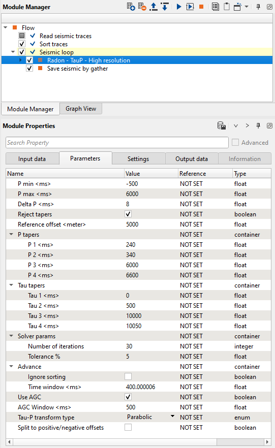
Figure 4. Job example with Radon - TauP parameters.
Interactive parameter testing that user can do on fly:
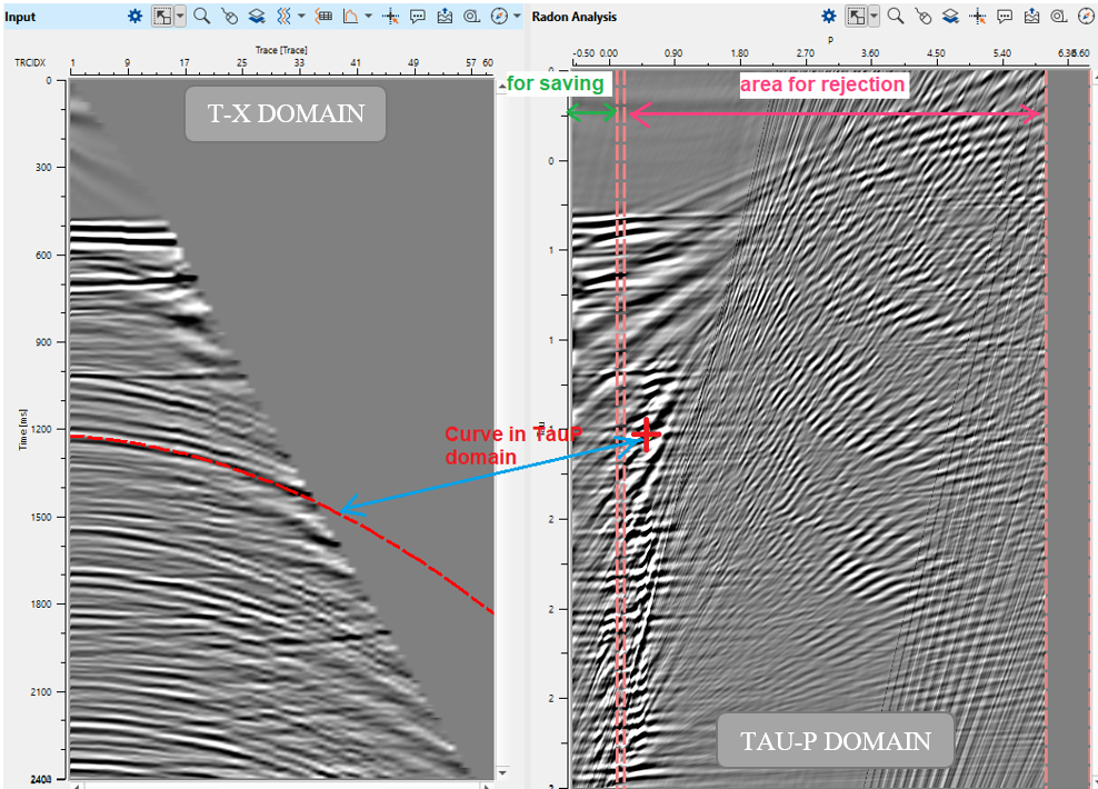
Figure 5. NMO-corrected CMP gather (left), its transform to the Tau-P domain (right).
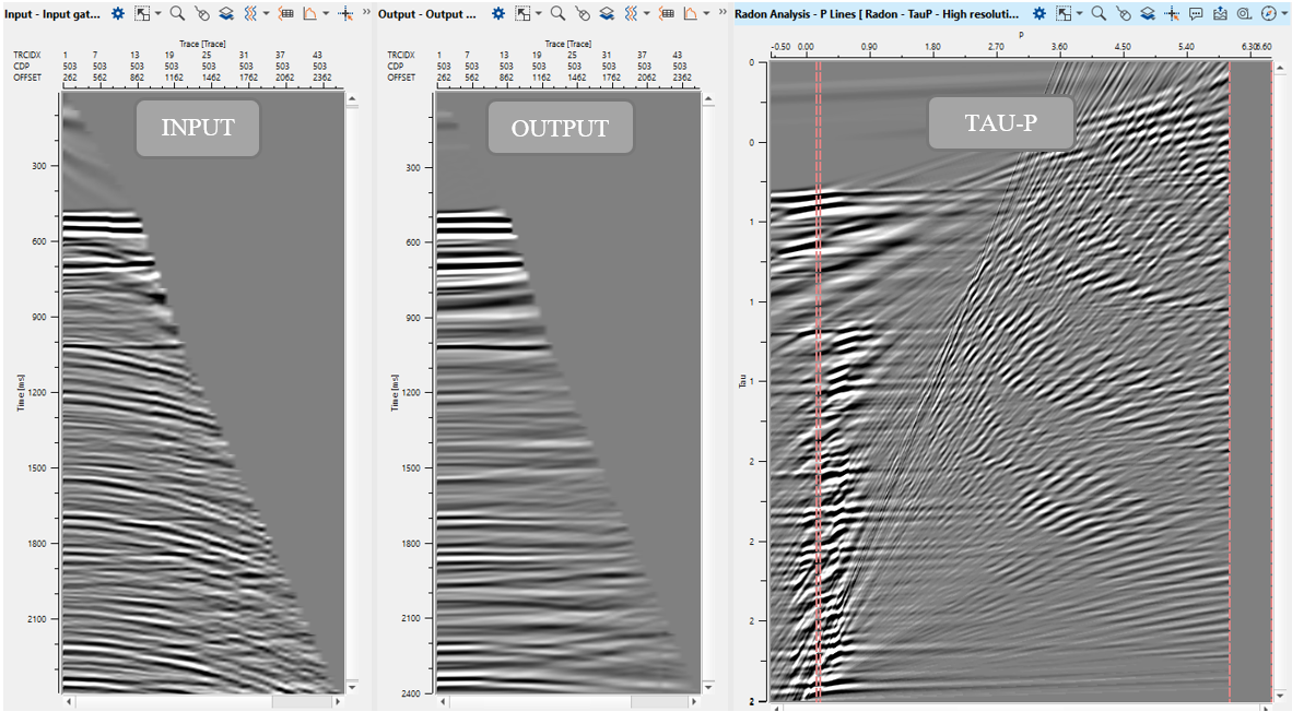
Figure 6. Quality control/Test parameters: Tolerance = 1%, Number of iterations = 2.
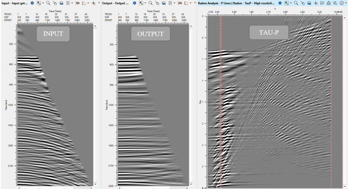
Figure 7. Quality control/Test parameters: Tolerance = 5%, Number of iterations = 2.
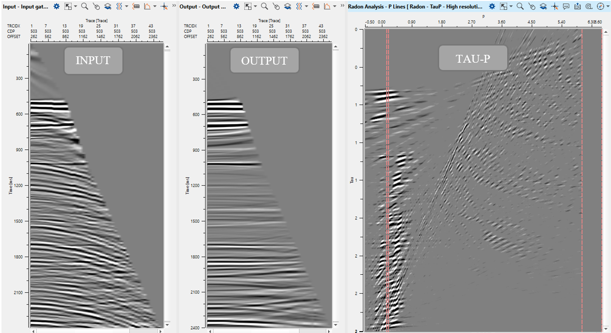
Figure 8. Quality control/Test parameters: Tolerance = 5%, Number of iterations = 32.
Interactive quality control on seismic gather (before and after) that user can do on fly:

Figure 9. NMO-corrected CMP gather: Input (left), Output (right).

Figure 10. Velocity spectrum before multiple attenuation (left) and after (right).
![]()
![]()
YouTube video lesson, click here to open [VIDEO IN PROCESS...]
![]()
![]()
Alvarez, G., 1995, A comparison of moveout-based approaches to the suppression of ground-roll and multiples: MSc Thesis, Colorado School of Mines.
Anderson, J., 1993, Parabolic and linear 2-D tau-p transforms using the generalized Radon transform: CWP Project Review.
Claerbout, J. F., 1995, Imaging the earth's interior: Blackwell Scientific Publications.
Hampson, D., 1986, Inverse velocity stacking for multiple elimination: Journal of the Canadian Society of Exploration Geophysicists.
Yilmaz, O., 1987, Seismic data processing: Society of Exploration Geophysicists.
Neil Hargreaves, Nick Cooper & Peter Whiting (2001) High-Resolution Radon Demultiple, ASEG Extended Abstracts.
 If you have any questions, please send an e-mail to: support@geomage.com