![]()
![]()
One of the foremost important aspects of seismic data processing is to know the quality of the data. It can be done by various QC tools. During the marine seismic data acquisition, there are QC tools to measure the amplitudes of the seismic data in real time. These amplitude QC plots help the users to understand the quality of the seismic data. It helps to find out any problem in the streamer with respect to weak or dead hydrophone/channel, very higher amplitudes with a big change in the amplitude, any missing shots and/or channel(s) etc. RMS amplitude plots are very useful in assessing the quality of the data quickly.
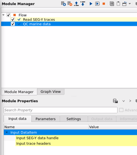
In g-Platform, we've a module called "QC marine data", wherein the user provides seismic data as an input to generate the RMS amplitude plots. This is one of the preliminary QC of the seismic data prior advancing to further data processing. These plots give a detailed understanding of the RMS amplitudes of the data. Based on this, the user can mark any noisy/spiky channels and cross check with the observer logs information.
![]()
![]()
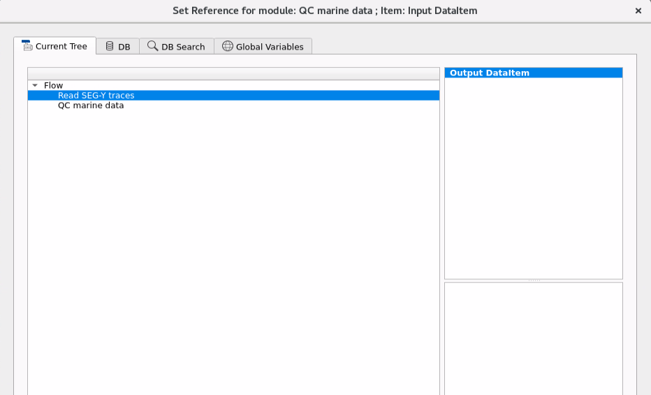
Input SEG-Y data handle - Make a reference to the Output SEG-Y data handle of Read SEG-Y Traces module.This is the only mandatory reference for QC marine data module.
Input trace headers - Reference to Output trace headers of Read SEG-Y Traces module.
Input DataItem - In other way, the user can directly reference the Input Dataitem to Output dataItem of "Read SEG-Y traces" module which considers both the Output SEG-Y data handle and Output trace headers.
![]()
![]()
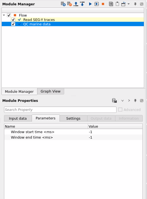
In this example below, we are showing the default parameters. The user can experiment with different start and end parameters to calculate the RMS amplitudes and generate the plots to better understand the seismic data quality.
Window start time - In order to calculate the RMS amplitudes, provide the window starting time in milliseconds (ms).By default -1 which means it'll take the entire trace length.
Window end time - Provide the end time of the calculated window to calculate the RMS amplitude. By default -1.
To generate the QC items, right click on QC marine data module-> Vista Groups-> All Groups-> In new window
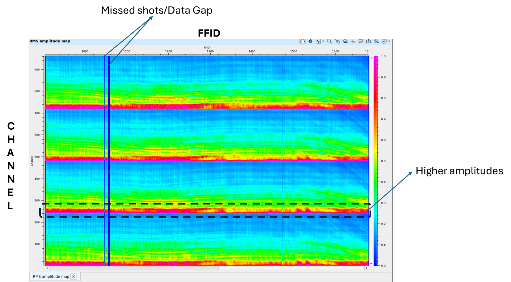
In the above RMS QC plot, we observe that there are 4 cables/streamers existing in this particular sail line. Each cable/streamer has got 240 channels. In the above plot, channels are plotted in vertical axis and FFIDs are plotted in Horizontal axis. On the right hand side, we can observe the color bar annotated with amplitude color range from 0 to 1. The user can change these color bar values by going to the View Properties of the QC marine data module.
It can be interpreted from the above RMS QC plot that there are missing shots between 1000 and 1100 FFIDs. This can be cross checked with the observer logs to confirm prior proceeding further. Also, at the near offset/channels of the each cable/streamer, there is high amplitude trend throughout the sail line. Likewise, if any channels are missing, we can see a horizontal line as it was showed for missing shot point/FFID.
![]()
![]()
Auto-connection - By default Yes (Checked). Whenever the module is present inside the Seismic loop, it will automatically reference the output of the previous module to the next modules input.
SegyReadParams
Bulk size - Number of traces to be processed in a bulk. By default 1000
Number of threads - One less than total no of nodes/threads to execute a job in multi-thread mode.
Skip - By default, No (Unchecked). This option helps to bypass the module from the workflow.
![]()
![]()
There are no Output data from this module because of that the Output data tab is disabled/grayed out.
![]()
![]()
Here is an example workflow to calculate the RMS QC plots for a single sail line with 4 cables/streamers of 240 channels each. In this example, we are calculating the RMS amplitudes for the entire trace length. So, we kept the starting and ending window to "-1" which means it considers the entire trace length.
![]()
![]()
YouTube video lesson, click here to open [VIDEO IN PROCESS...]
![]()
![]()
Yilmaz. O., 1987, Seismic data processing: Society of Exploration Geophysicist
 * * * If you have any questions, please send an e-mail to: support@geomage.com * * *