Time Varying Gain (TVG)
![]()
![]()
Seismic signals/traces travel through the sub-surface experiences energy loss. This energy loss is due to various factors. Due to the near surface conditions, environmental factors. When the seismic energy source is fired, the energy passes through the sub-surface. During this process, the seismic trace loses energy by means of geometrical spreading, absorption, scattering etc.
The distance between source-receiver plays an important role. As the signal travels from the source side to the receiver side, the time it takes to reach the receiver plays an important role. As the travel time increases the energy loss is also increases. Due to this, the deeper events lack the proper amplitudes when compared to the shower events. All the energy is concentrated at the shallower events. To compensate these energy losses, there are various techniques are used in the seismic data processing. Out of those, Time-Varying Gain is one of them.
Time-varying Gain is used to compensate the natural attenuation of the seismic signal. It is used to restore the amplitudes of the seismic signal as the waves pass through the sub-surface it loses the energy and there a huge difference of amplitudes between the shallower and deeper events. This time varying gain compensates the lower amplitudes in the deeper regions.
Time-varying Gain adjusts the amplitudes of the seismic signal based on the time traveled from the source to the receiver. This is performed by using spherical divergence gain, exponential gain and power-law gain.
The basic mathematical principal of the time-varying gain is pretty simple.
The typical gain function equation be like g(t) = A*Tn where
g(t) - Gain function at time t
A - Scaler which is usually 1
T - travel time from the source to the receiver
n - exponent. This controls how quickly the gain increases with time.
![]()
![]()
Input DataItem
Input gather - Connect/reference to the input data gather. If it is inside the seismic loop, it will automatically connects the previous modules output gather as input gather to this Time-varying Gain module.
![]()
![]()
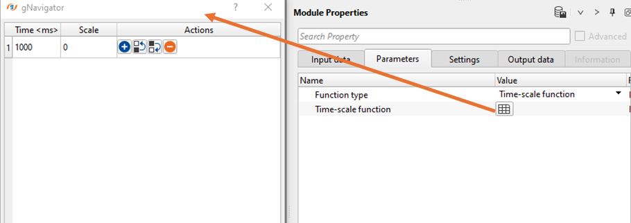
Function type { Time-scale function, Trace coefficient, Scale by trace header, Trace headers expression }
Time-scale function - It is a mathematical function that describes how gain is applied to the seismic signals with varying time.
Time-scale function - This function varies as a function of time and it's purpose is to model how the amplitudes of the seismic signal varies with the time. Define the Time and Scale factors at different time intervals as shown in the below image.
As we know that the shallower region will have less energy loss compared to the deeper regions. So, we can define the Scalar factor accordingly. As we go to the higher travel times, the scale factor increases with the time.
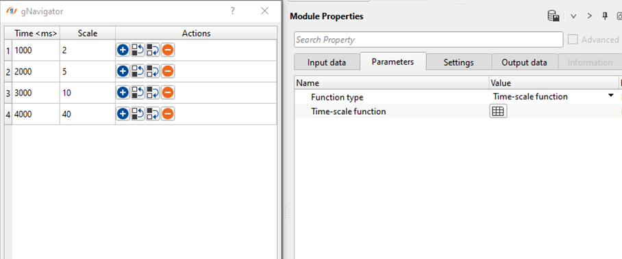
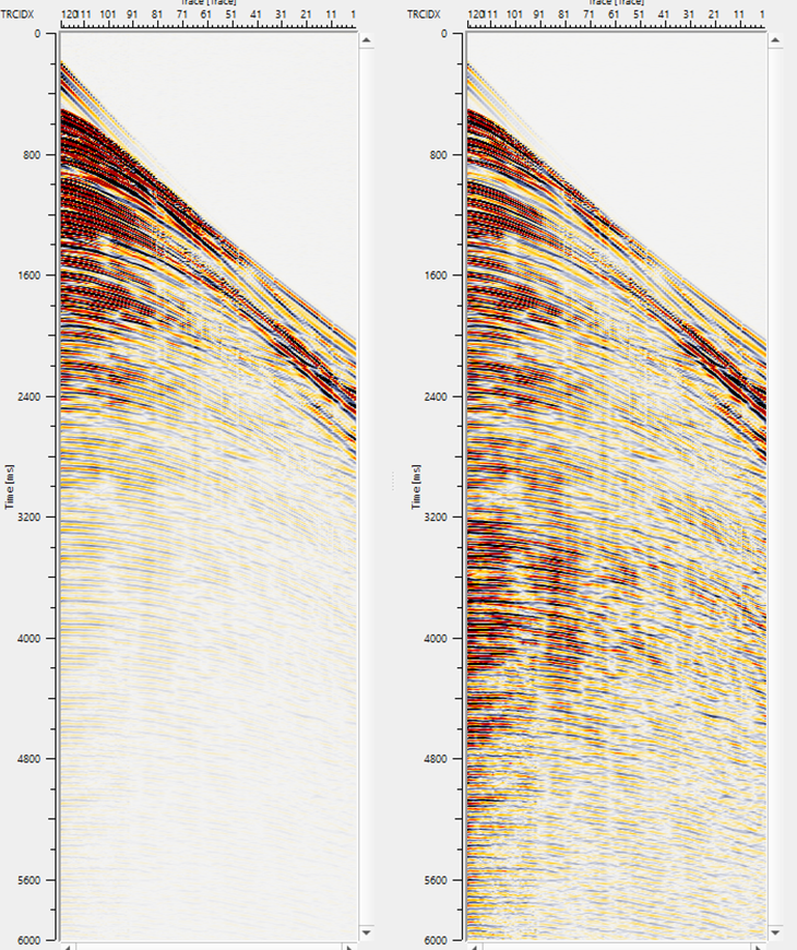
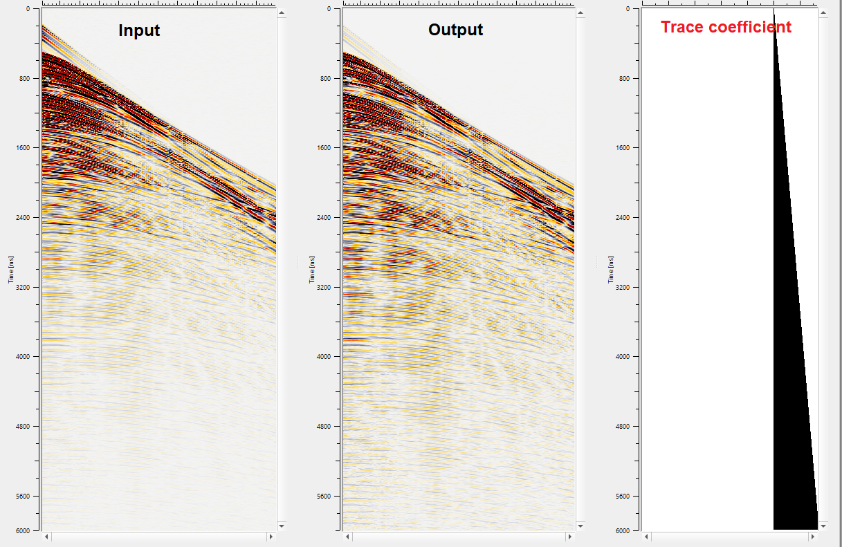
With the above Scale factor parameters, we can clearly see the energy compensation in the below image after application of TVG using Time-Scale Function.
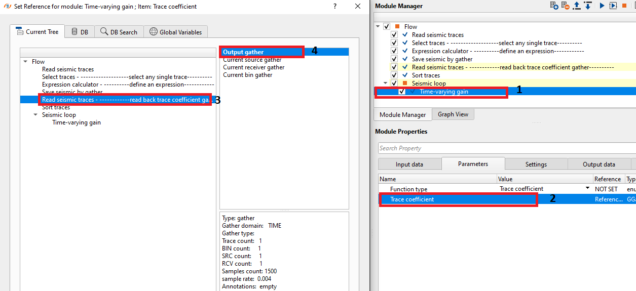
Trace coefficient - This is a scaler factor applied sample by sample to the entire trace. It varies with the variation in the time and it is applied to compensate the amplitude decay(energy loss) due to attenuation of the seismic energy source. Detailed explanation about the process is explained in the Examples section.
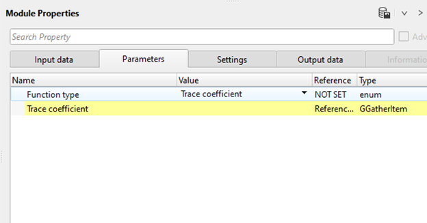
Trace coefficient - connect/reference to the output gather of "Read seismic trace" module.
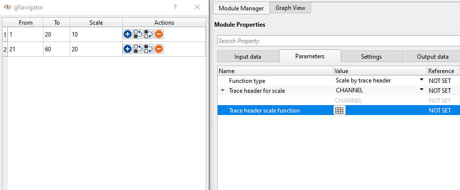
Scale by trace header - This refers to scaling factor applied globally to the seismic trace by using any trace header information. Seismic data trace headers store certain information like gain factor, scale factor etc in the trace headers. We can use this information to scale the trace headers or we can use any particular trace header and apply the scaler.
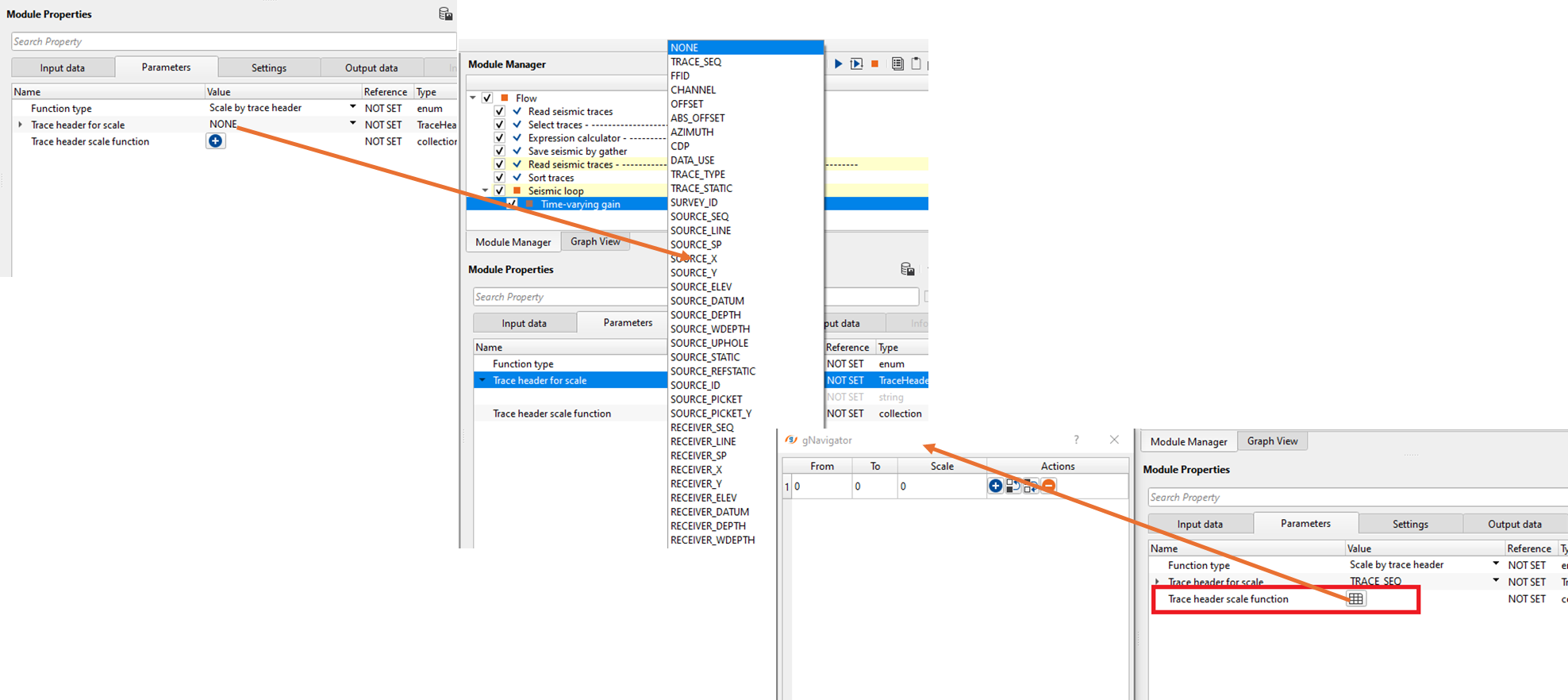
Trace header for scale - Select the trace header from the drop down menu.
Trace header scale function - specify the from and to values of the selected trace header and the corresponding scaler values.
Trace headers expression - By using any trace header expression, we can apply a scaler value to this. Here we can specify the window i.e. from & to time windows. Along with it, we've to provide the trace header expression. We can add multiple rows here and choose different expressions.
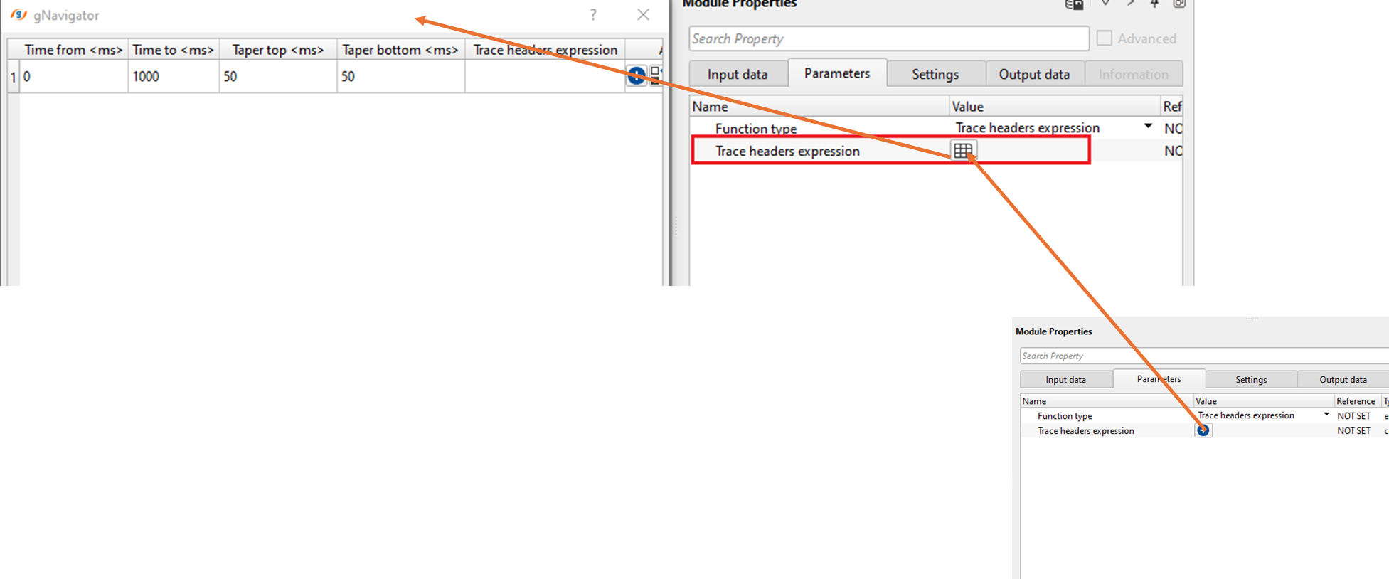
Trace headers expression - Specify the trace header expression to a particular time window and the corresponding scaler value.
![]()
![]()
Auto-connection - By default Yes (Checked)
Bad data values option { Fix, Notify, Continue } - This is applicable whenever there is a bad value or NaN (Not a Number) in the data. By default Notify. While testing, it is good to opt as Notify option. Once we understand the root cause of it, the user can either choose the option Fix or Continue. In this way, the job won't stop/fail during the production
Calculate relation - When checked this option, it will calculate the amplitude relation.
Number of threads - One less than total no of nodes/threads to execute a job in multi-thread mode.
Skip - By default, No (Unchecked). This option helps to bypass the module from the workflow.
![]()
![]()
Output DataItem -
Output gather - Outputs the time varying gain applied output gather.
Amplitude relation - It will output the amplitude relation
![]()
![]()
In the below, we are explaining how the trace coefficient, scaling by trace header works.
Here is he procedure to generate the trace coefficient.
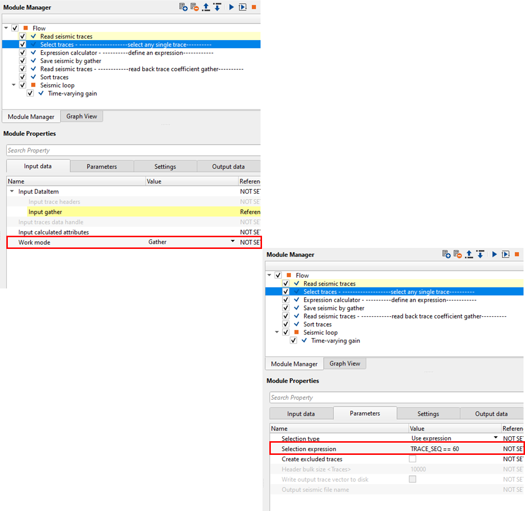
•The user should have a single trace (can select any trace from the input gather by using Select traces module).
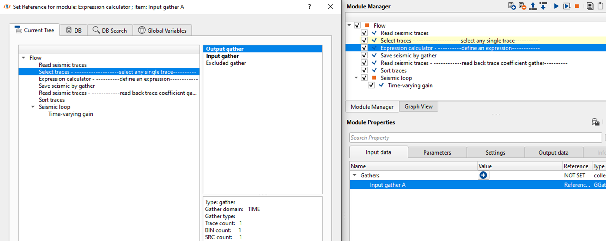
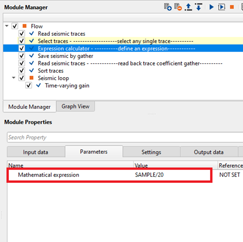
•Use "Expression Calculator" module and define an expression to get the trace coefficient. In this example, we are defining an express as "SAMPLE/10". What it does is, it generates a trace coefficient for each sample. This trace coefficient will be multiplied with the each sample of the seismic trace and compensate the gain.
•Save this trace coefficient by using "Save seismic by gather" module.
•Read back the trace coefficient by using "Read seismic traces" and load data to RAM as YES
•Connect/reference the Trace coefficient to Output gather of Read seismic traces.
In case the trace coefficient is provided by the client then use any one of the read seismic data modules and connect with the trace coefficient parameter.
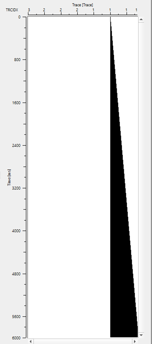
Output from the Expression calculator. This is the trace coefficient as shown in the below image.
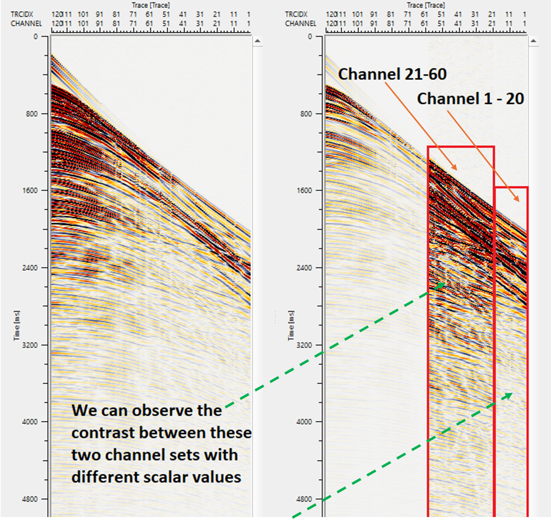
Scale by Trace header - In this example, We've chosen Channel as the trace header and we would like to apply different scalars for different channels.
Trace headers expression - In this method, the user should provide the area where the gain should be applied with an trace header expression. Also, it gives the option for the user for a smooth transition of the gain above and below the applied zone.
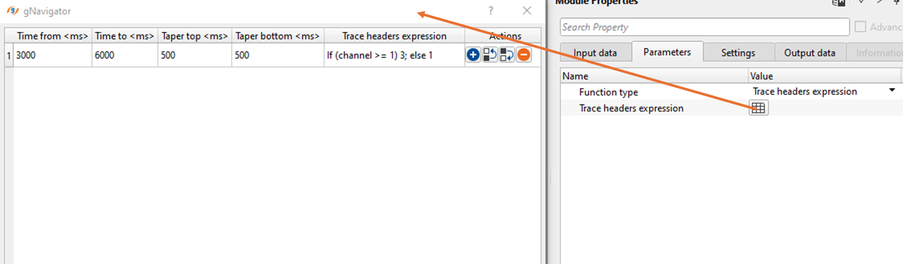
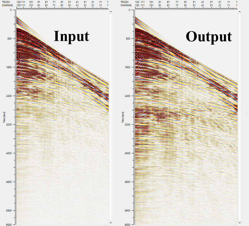
In the above image, we can see the time start and time end with top and bottom tapers. In the trace headers expression column, we've defined that channel > = 1, it should multiply the coefficient with 3 else keep the value as 1. This will increase the amplitudes within the user specified window i.e. from 3000 - 6000 ms with a taper of 500 ms on above and below the specified window. The resultant output is shown below.
![]()
![]()
There are no action items available for this module so that user can ignore it.
![]()
![]()
YouTube video lesson, click here to open [VIDEO IN PROCESS...]
![]()
![]()
Yilmaz. O., 1987, Seismic data processing: Society of Exploration Geophysicist
 * * * If you have any questions, please send an e-mail to: support@geomage.com * * *