Change domain of horizon from time to depth (PSDM stage)
![]()
![]()
This module converts interpreted horizons from the time domain into the depth domain using an interval velocity model. Horizon data is typically delivered by an interpretation team as text files containing three columns: the X coordinate, the Y coordinate, and the picked two-way travel time (t0) at each location. The module supports three horizon input modes: ASCII files on disk, internal g-Platform horizon items (connected from other modules), and interpolation matrices created in the Create Interpolation Matrix module.
The conversion is performed by ray-tracing downward through the interval velocity model at each survey location. For each trace position in the velocity gather, the module accumulates one-way travel time sample by sample through the depth velocity profile until the horizon time is reached; the corresponding depth value is then recorded using linear interpolation between samples. This approach correctly accounts for lateral velocity variations across the survey area.
This module is a key step in the Pre Stack Depth Migration (PSDM) workflow. The resulting depth horizons can be used directly as input to the VTI Epsilon Estimation module for anisotropic parameter analysis, or for other depth-domain interpretation tasks. Both a depth-domain and a time-domain version of each horizon are produced as outputs.
![]()
![]()
There is no parameters here (please, find input horizon files and velocity in the parameters tab).
![]()
![]()
Velocity import type { Gather, Files } - select type of input interval velocity model (depth domain): gather or SEGY file on a disk.
Choose how the interval velocity model (in the depth domain) is supplied to this module. Select Gather to connect a velocity gather directly from an upstream module in the workflow — for example, from a velocity model builder or a Load Item module. Select Files to read the velocity model from one or more SEG-Y files stored on disk. The velocity model must be in the depth domain (interval velocities as a function of depth), not in the time domain.
Input files velocity - if Files is selected: select SEGY file of input interval velocity model (depth domain).
Visible only when Velocity import type is set to Files. Add one or more SEG-Y files containing the interval velocity model in the depth domain. Each file should contain traces whose samples represent interval velocity values (in m/s) at successive depth levels. The sample interval of the velocity gather defines the depth step used during ray-tracing. Multiple files can be added if the velocity model is split across several files covering different parts of the survey area.
Depth velocity - if Gather is selected: select SEGY file of input interval velocity model (depth domain).
Visible only when Velocity import type is set to Gather. Connect the interval velocity gather from an upstream module in the processing workflow. The gather must contain depth-domain interval velocity data, where each trace represents a single surface location and each sample holds the interval velocity (m/s) at the corresponding depth. The geometry (X, Y coordinates and datum) embedded in the velocity gather is also used to define the spatial grid for the depth conversion output.
Horizons type { Item, Files, Matrices } - select type of input horizon (time domain): item is a internal data type that can saved and imported from the g-Platform data base, file on a disk or matrix (this is type of map that can be created in Create interpolation matrix module).
Choose how the input horizon (in the time domain) is provided. Item connects a horizon picking item directly from another module in the workflow, such as a Load Item or a picking module. Files reads horizon data from ASCII text files on disk — each file must contain exactly three whitespace- or semicolon-delimited columns per line: X coordinate, Y coordinate, and the picked two-way travel time value (t0). Lines that do not contain numeric data are automatically skipped. Matrices uses a regularly gridded time map created by the Create Interpolation Matrix module, which already holds time values at each grid node.
Input files horizons - select SEGY file on a disk: input interval velocity model (depth domain).
Visible only when Horizons type is set to Files. Add one or more ASCII horizon files (extensions .hor or .txt). Each file should contain three columns per data line: X coordinate, Y coordinate, and the horizon time value. The file name (without extension) is used as the layer name in the output horizon item. Multiple files can be added to convert several horizons in a single run — each file becomes a separate layer in the output.
Input time horizons - connect horizon Item data type from Load item module or from specific module that generates this type of data.
Visible only when Horizons type is set to Item. Connect a g-Platform horizon picking item from an upstream module, such as a Load Item node or a horizon picking module. The item may contain multiple named horizon layers; each layer is converted independently and appears as a corresponding layer in the output depth horizon item.
Input matrices - connect matrix from specific module that generates this type of data (Create interpolation matrix).
Visible only when Horizons type is set to Matrices. Connect one or more named matrix items produced by the Create Interpolation Matrix module. Each matrix holds a regular grid of time values representing a horizon surface. Assign a name to each matrix entry — this name labels the corresponding layer in the depth output. The matrix grid step is read automatically from the matrix itself and does not need to be re-entered here.
V0 - define velocity (m/s) in a low velocity zone (weathering zone).
Set the propagation velocity (m/s) in the near-surface low-velocity zone (the weathering layer) above the datum. This value is used to compute the travel-time correction that accounts for the elevation difference between the topographic surface and the processing datum plane. If the datum and the topographic surface coincide, or if the velocity model already starts at the surface, this parameter has no effect. The default value is 2000 m/s, which is a typical replacement velocity for consolidated near-surface sediments. Adjust this value to match the actual near-surface velocity at your survey location.
Trace step to fit - module get this amount of traces for conversion from time to depth, i.e. chunk by chunk in accordance with geometry (which is read from velocity gather) recommendation is to keep it by default is 50 traces.
Controls the spatial density of depth-conversion points drawn from the velocity gather. A value of N means that every N-th trace in the velocity gather is used for the ray-tracing calculation; the computed depth values at those locations are then interpolated to fill the full output grid. Smaller values produce denser sampling and more accurate results at the cost of longer processing time; larger values speed up computation but may miss lateral velocity variations. The default value of 50 is appropriate for most surveys where the velocity model varies smoothly. Reduce this value (for example, to 10–20) if the velocity model has significant lateral changes over short distances.
Import horizons from ASCII params - parameter for horizons file importing:
This group of parameters controls how time values in the input ASCII horizon files are interpreted before depth conversion. Use these settings to specify the reference datum level, apply a unit scaling factor to the time values, and add any constant shifts in time or depth that may be needed to align the horizon with the velocity model.
Location { Datum, Topography } - select the datum type on what level horizon is located: constant of elevations.
Specifies the reference surface from which the horizon time values are measured. Select Datum if the picked times are two-way travel times measured from a constant flat datum plane (the standard case for most processed seismic data). Select Topography if the times are measured from the actual ground surface elevation at each point (as in some field-acquired data or refraction picks). Choosing the wrong option will introduce a systematic depth error equal to the datum-to-surface travel-time correction.
Datum - if Datum option is selected define a constant datum plane value in meters.
Active only when Location is set to Datum. Enter the elevation of the flat datum plane in meters (positive upward from sea level). This value must match the datum used during seismic processing to ensure the time-to-depth conversion reference is consistent. The default is 0 m (sea level). Valid range: -1000 m to 100000 m.
Scalar - if necessary, scalar coefficient that will be applied to time values.
A multiplicative scale factor applied to all time values read from the ASCII horizon files before depth conversion. The default value is 0.001, which converts milliseconds (the typical unit in ASCII horizon exports) to seconds (the unit expected internally for ray-tracing against the depth velocity model). If your horizon file already contains values in seconds, set this to 1.0. If your file contains values in a different unit or requires a polarity correction, adjust this scalar accordingly.
Add constant shift time - if necessary add a constant shift in milliseconds to the horizon.
Adds a constant value (in milliseconds) to all horizon time picks before the depth conversion is performed. Use this to correct for a known bulk time shift between the horizon picks and the seismic data — for example, if the interpretation was done on data with a different static correction applied. A positive shift moves the horizon to a later time (greater depth); a negative shift moves it to an earlier time. The default is 0 ms (no shift).
Add constant shift depth - if necessary add a constant shift in meters to the horizon.
Adds a constant value (in meters) to all computed depth values after the time-to-depth conversion. Use this to apply a bulk depth correction — for example, if a known depth offset exists between the converted horizon and well tops or other depth control. A positive value shifts the horizon deeper; a negative value shifts it shallower. The default is 0 m (no shift).
Map interpolation - define interpolation method and parameters for horizon map creation from input grid (points item):
This group of parameters controls how the scattered depth-converted horizon points are interpolated onto a regular output grid. After depth conversion, the module has a set of depth values at discrete velocity trace locations. These are gridded using the chosen interpolation algorithm and output grid steps to produce a smooth, spatially continuous horizon surface.
Interpolation type { Kriging, ABOS } - algorithms for map interpolation: Kriging, ABOS.
Select the spatial interpolation algorithm used to grid the depth-converted horizon points onto the output map. ABOS (the default) is a fast distance-weighted interpolation method that works well for most surveys with reasonably uniform data coverage. Kriging is a geostatistical method that uses a spatial covariance model to produce a statistically optimal estimate; it can better handle irregular data distributions and provides smoother results in areas of sparse coverage, but requires additional configuration of covariance parameters.
Kriging covariance { Spherical, Gaussian, Exponential } - - the covariance type refers to the mathematical model used to describe the spatial correlation between data points. This covariance model plays a crucial role in defining how the values at different locations are statistically related, which directly impacts the interpolation results.
Active only when Interpolation type is set to Kriging. Selects the covariance (variogram) model that describes how spatial correlation between horizon depth values decreases with distance. The default is Spherical, which is suitable for most geological horizons with a definable correlation range. Use Gaussian for very smoothly varying horizons. Use Exponential for data where spatial correlation drops off rapidly with distance.
Exponential - Suitable for data with rapidly decreasing spatial correlation. Correlation diminishes exponentially with distance but never truly reaches zero.
Spherical - A commonly used covariance type that assumes the spatial correlation increases up to a certain distance (called the range), beyond which points are uncorrelated. The correlation gradually decreases as the distance approaches the range.
Gaussian - Represents a smooth, gradual decrease in correlation, often used for very continuous data.
Kriging range - parameter of the variogram or covariance model that defines the maximum distance over which spatial correlation exists between data points. Beyond the range, the values at different locations are considered uncorrelated or independent.
Active only when Interpolation type is set to Kriging. Sets the maximum distance (in meters) over which data points influence each other during kriging interpolation. Points separated by more than this distance are treated as spatially independent. The default is 100000 m. Set this value to approximately the spatial scale over which you expect the horizon depth to vary smoothly — typically similar to the average distance between horizon picks in your dataset. Minimum value: 1 m.
Kriging max points - refers to the number of nearby data points used to estimate the value at an unknown location during the interpolation process. This parameter controls how many known values in the vicinity of the target point are included in the kriging calculation.
Active only when Interpolation type is set to Kriging. Limits the number of nearest neighbor points used in each kriging estimate. Using fewer points reduces computation time; using more points increases accuracy but slows down the interpolation. The default is 50 points, which is suitable for most surveys. Minimum value: 1.
Interpolation step X - step in meters for the interpolation along X axes.
Sets the output grid node spacing (in meters) along the X direction for the interpolated depth horizon map. A finer step produces a higher-resolution output map but requires more memory and computation time. A coarser step is appropriate when the input horizon picks are sparsely distributed. The default value is 150 m. Set this to match the typical bin spacing of your seismic survey or the resolution of the velocity model. Minimum value: 1 m.
Interpolation step Y - step in meters for the interpolation along Y axes.
Sets the output grid node spacing (in meters) along the Y direction for the interpolated depth horizon map. This should be set consistently with Interpolation step X. For surveys with approximately equal bin dimensions in X and Y, use the same value for both. The default value is 150 m. Minimum value: 1 m.
![]()
![]()
Number of threads - limit number of threads on main machine.
Controls the maximum number of CPU threads used for parallel processing during the depth conversion and map interpolation steps. Increasing the thread count speeds up computation on multi-core machines. Set this to the number of physical cores available on your workstation for best performance, or leave it at the default to allow g-Platform to use all available cores automatically.
Skip - switch-off this module (do not use this module in the workflow).
When enabled, this module is bypassed entirely and passes its inputs through to the next module in the workflow without performing any processing. Use this option to temporarily disable the depth conversion step for testing or troubleshooting purposes, without needing to disconnect and reconnect the module in the workflow graph.
![]()
![]()
Output depth horizons - horizon item in depth domain that can be used in VTI epsilon estimation.
The primary output: a g-Platform horizon item containing the converted horizon surfaces in the depth domain (meters). Each input horizon layer appears as a named layer in this output item, preserving the original horizon names. This item can be connected directly to the VTI Epsilon Estimation module as input, or saved to the g-Platform database for later use. The depth values are defined on the interpolated output grid with the step sizes specified by Interpolation step X and Interpolation step Y.
Output time horizons - horizon item in time domain.
A secondary output: a g-Platform horizon item containing the same horizon surfaces in the time domain, gridded and interpolated onto the same output spatial grid. This time-domain output is produced alongside the depth output and allows comparison between the original time picks and the interpolated time surface at the same grid resolution. It also serves as a quality-control tool to verify that the input time picks were read and interpolated correctly before examining the depth conversion results.
![]()
![]()
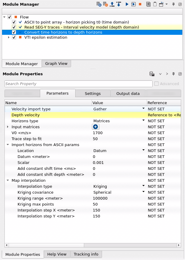
Example of the workflow: read depth velocity model as gather and horizon picking from ASCII file, then convert horizon time domain t0 to depth domain h0:
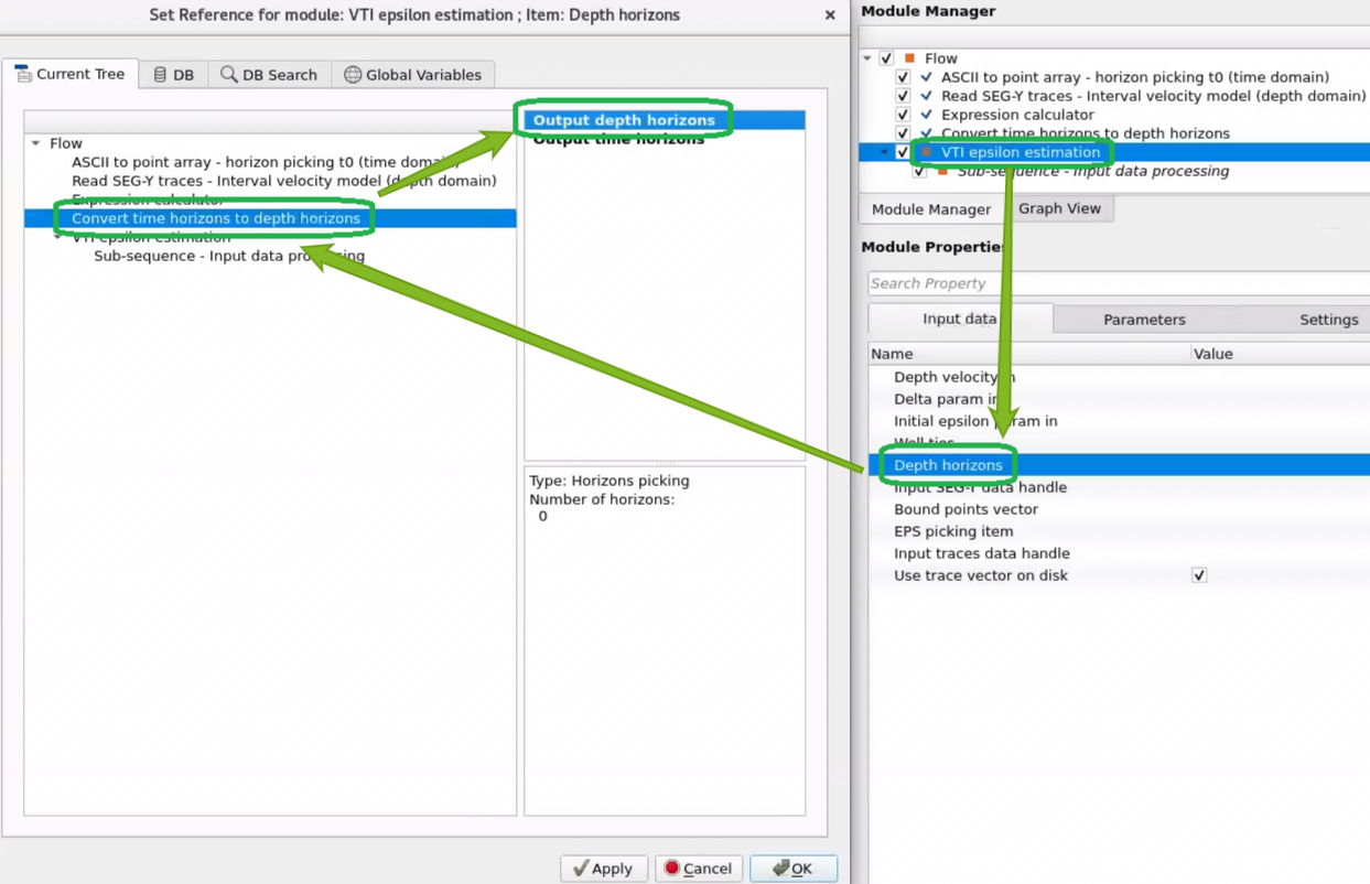
Resulting horizon in depth domain can be used in the VTI epsilon estimation module as input data:
![]()
![]()
YouTube video lesson, click here to open [VIDEO IN PROCESS...]
![]()
![]()
 If you have any questions, please send an e-mail to: support@geomage.com