Reading SEG-Y traces
![]()
![]()
Read SEG-Y traces module is designed to read seismic traces from SEG-Y files, and make them available to use inside g-Platform.
In addition to reading in all the traces of a SEG-Y, this module can also be used for the following:
•Adjust trace headers with mathematical expressions (Trace Header Dictionary)
•Read traces according to trace type
•Recalculate offsets according to coordinates
•Load all traces directly to RAM memory for use as a gather input (NOTE: This should only be done with small SEG-Y. See “load Data to RAM” for more information).
Read Seg-y traces will not be used for displaying the input traces SEG-Y data, even when the module has run successfully. To view seismic data, there are different ways to use Read SEG-Y traces module to display the data.
Enable active location map - It will display the gathers when the user selects them on the location map.
Load data to RAM - This will be used ONLY when the input data size is small. We DO NOT recommend for large dataset(s).
For more detailed information about Enable active location map & Load data to RAM, it is described in EXAMPLES section.
How to create new trace header format?
Geomage format is a standard SEG-Y Rev 1.0. This is the default trace header format inside the Read SEG-Y traces module. User can create a new trace header format as per the input data requirements.
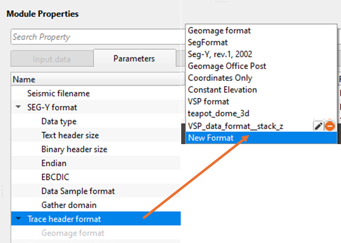
•Go to Trace header format and click on Geomage format.
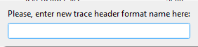
•At the bottom of the drop down menu, New format exists. Click on New format. Give it a name.
•Now the Trace header format changes from Geomage format to user defined format.
•Click on the calculator/table icon. It will open a window. Edit the trace headers as per the input data.

How to change Trace Headers with mathematical expressions in the Trace Header dictionary?
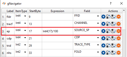
Use the “Expression” Column to modify incoming trace headers. Trace headers are modified according to their byte location. The adjusted trace headers will be take the place of the trace header indicated by the field column.
Use the format as Item Type(Start Byte).
Item type - Int4, Float4, Int2, Float2 etc.
Start Byte - starting byte location of the corresponding trace header.
Examples of mathematical expressions used within the trace header format.
Divide incoming SOURCE_SP by 100
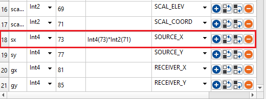
Multiply a coordinate value by the coordinate scalar included in the trace headers:
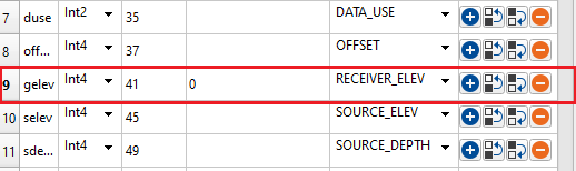
Set every value of for a trace header to a single value
•Use any valid mathematical operation or function to modify trace headers
oMathematical operators (+, -, *, /, %, ^)
oFunctions (min, max, avg, sum, abs, ceil, floor, round, roundn, exp, log, log10, logn, root, sqrt, clamp, inrange)
oTrigonometry (sin, cos, tan, acos, asin, atan, atan2, cosh, cot, csc, sec, sinh, tanh, d2r, r2d, d2g, g2d, hyp)
•Change Start byte to match the appropriate value in the Field column. Don’t change the value in Field to match the start byte.
![]()
![]()
Input data tab is disabled for this module. All the input data MUST be provided in the Parameters tab.
![]()
![]()
Seismic filename - provide full path and file name of the input SEG-Y
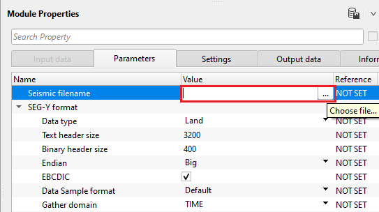
Click inside the Value field and click on "...". Provide full path and file name of the input SEG-Y.
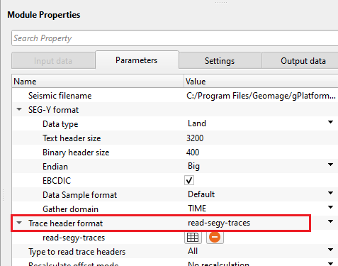
SEG-Y format - This section deals with the basic SEGY format details like type of data i.e. land/marine/transition, EBCDIC, binary headers information etc.
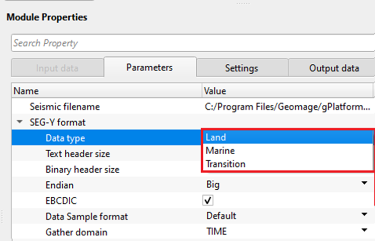
Data type - specify the input data type from the drop down menu. There are 3 types available. Land, Marine, Transition.
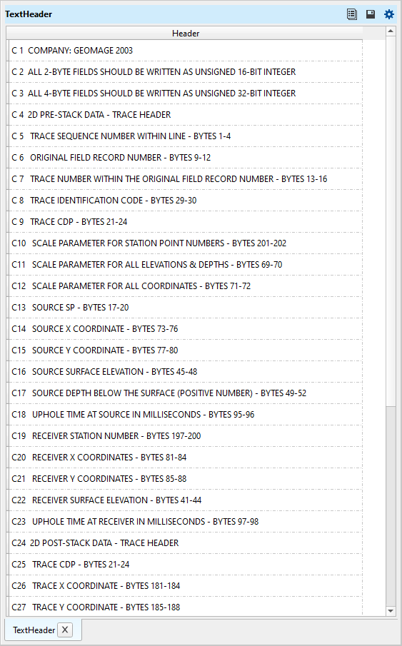
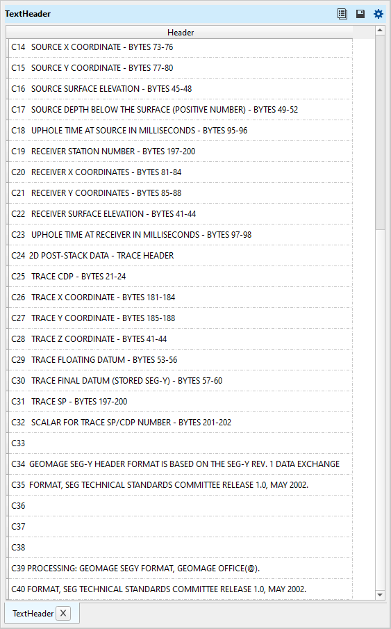
Text header size - text header stores the survey and processing history information. This is in ASCII format. The default size is 3200 bytes. This is also known as EBCDIC header. The standard size of the text header is 40 rows and 80 columns.
Binary header size - this header stores the data in binary format. Default size is 400 bytes. In this header, we get sample interval, no of samples, measurement system, data format (IBM, floating point, ....) etc. information is stored.
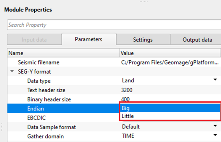
Endian - it refers to the byte order in which a computer stores the multi byte (integers, floating point etc) data in memory or files.
Big Endian - Most Significant Byte is stored at Lowest memory address. Most old computers used Big Endian.
Little Endian - Least Significant Byte is stored at Lowest memory address. Modern computes uses Little Endian.
EBCDIC - displays the EBCDIC/text header if this option is TRUE (Checked). By default, TRUE (Checked).
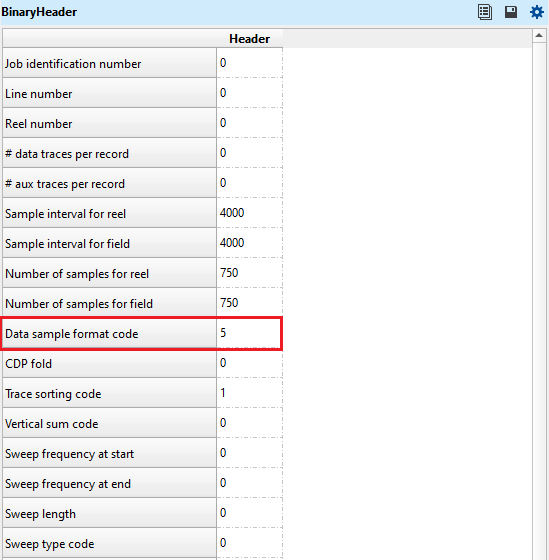
Data sample format - it represents the seismic trace amplitudes in binary format. It defined in 25-26 byte location of SEG-Y binary header. By default, IEEE (most modern systems uses this). Incorrect data sample format leads to wrong amplitudes, clipping of high/low amplitudes etc. It is also important that both data sample format and Endian type are accurate and correct.
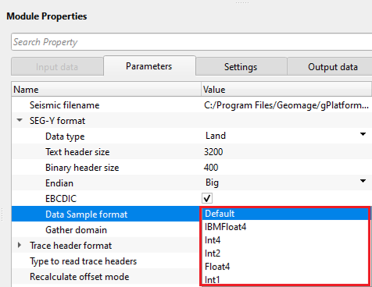
Default - IEEE format
IBMFloat4 - IBM 32 bit Floating point with 4 Bytes as sample size. Most legacy SEGY data is in this format.
Int4 - 32 bit Integer point with 4 Bytes as sample size.
Int2 - 16 bit Integer point with 2 Bytes as sample size.
Float4 - IEEE 32 bit Floating point with 4 Bytes as sample size. Modern SEGY data is in this format.
Int1 - 8 bit Integer point with 1 Byte as sample size.
How to check the correct data sample format?
Go to byte 25-26 byte location of SEG-Y binary header and look for the format IDs.
IBM Float - 1
IEEE Float - 5
Gather domain - allows the user to specify the input data domain type. By default, Time. There are additional domain options available from the drop down menu.
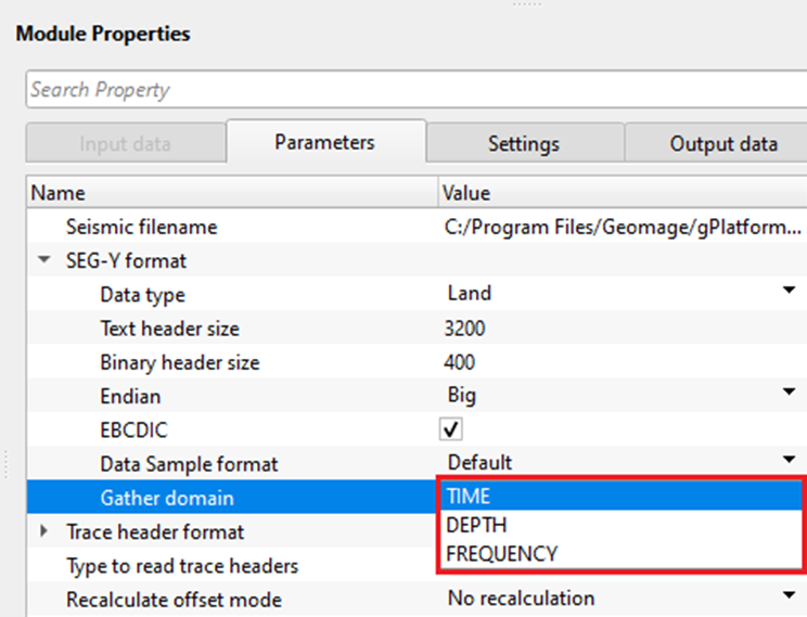
Time - Input data is in Time domain
Depth - Input data is in Depth domain
Frequency - Input data is in Frequency domain
Trace header format - it contains meta data of the seismic trace which means all the parameters like source point, FFID, channel number, source and receiver coordinates etc., are stored at certain byte locations. This is very crucial while reading the SEG-Y data. Make sure that the trace headers mapped correctly to their respective byte locations with correct format.
By default, Geomage format. This is a standard SEG-Y rev 1.0 format. Look for more detailed explanation in the EXAMPLES section.
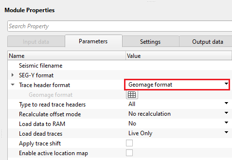
Type to read trace headers { All, First N, Each N } - specify to read all traces or first trace of each gather or each gather. By default, All. It reads all the traces.
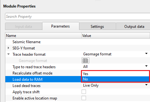
Recalculate offset mode { No recalculation, Recalculate as 2D, Recalculate as 3D } - - this allows to recalculate the offsets by using the source and receiver coordinate values. By default, No recalculation.
No recalculation - It won't calculate the offsets
Recalculate as 2D - It takes the source and receiver x,y coordinate values and calculates the offset
Recalculate as 3D - It is applicable to the 3D dataset. Similar to 2D, it computes the offsets by using source and receiver x,y coordinates.
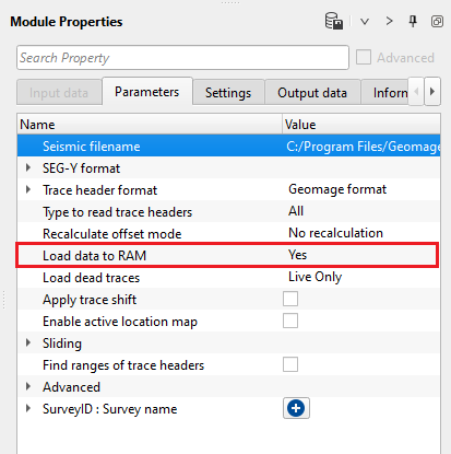
Load data to RAM { Yes, No } - this allows the input data to be displayed as Output. By default, NO. To display the entire input dataset, Load data to RAM as YES. Look for more detailed explanation in the EXAMPLES section.
![]() We recommend NOT to use YES option if the input data size is too big.
We recommend NOT to use YES option if the input data size is too big.
Load dead traces { All traces. Mute dead traces, Live Only, Dead Only, All traces } - this allows the user to decide what kind of traces to be read. Seismic traces have a trace identification number in their trace headers. Based on this, it'll decide whether to read all traces or leave the dead traces.
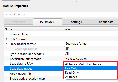
All traces, Mute dead traces - reads all the input traces but mutes/deletes the traces with a trace identification as dead (2)
Live only - reads traces with a trace identification as live (usually 1). By default, Live only.
Dead only - reads Dead traces with trace identification as Dead (2)
All traces - reads all the input traces
Apply trace shift - this allows to apply trace shift to each trace if any trace shift value is stored in the trace headers. By default, FALSE (Unchecked).
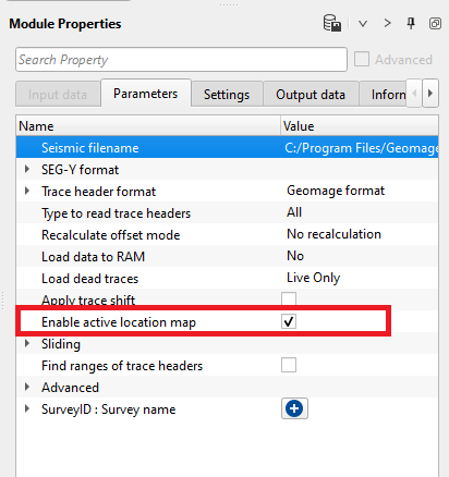
Enable active location map - This allows the user to display the gathers (source/receiver/bin). By default, FALSE. Look for more detailed explanation in the EXAMPLES section.
Sliding - this section deals with the seismic data animation settings i.e. moving a gather with a certain step size with certain amount of speed or delay.
Step - specify the interval between one gather to the next gather. For example, if the step size is 2 then it will display every 2nd gather.
Delay - specify the time delay that needs to be maintained between gathers while they are displaying. If the delay time is 100ms then it will pause for 100ms before displaying the next gather.
Slide BIN - it will moves the bin gather.
Slide SRC - it will moves the source gather.
Slide RCV - moves the receiver gather.
Find ranges of trace headers - by default, FALSE (Unchecked). If this option is TRUE (Checked), it scans through the entire input dataset and finds out minimum and maximum values of each trace header. All the ranges of trace headers information is available in the "Information" tab.
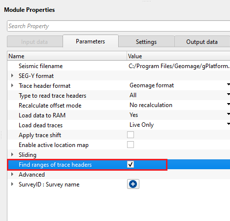
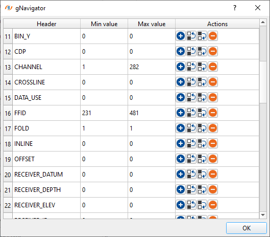
Click the table icon of the Trace headers and it open a new window with all trace headers information.
Advanced - this deals with additional parameters which are not mandatory however it is important to pay attention to some of the parameters like Datum etc.
Number of traces - total number of traces to be read as a bulk. By default 100000
Load raw headers - by default, FALSE (Unchecked). It'll load all the raw trace headers.
Distance for merging points - determines the distance where various source\receiver points will be merged to one point. By default, 0.1 meters.
Apply weight - If this check box is checked, then amplitude weight written in trace header will be used for each trace.
Data datum { Datum trace header, Topography, Constant datum } - choose the correct datum type while reading the data. In case, input data(post stack) having datum information in the trace headers, read the datum from datum trace header.
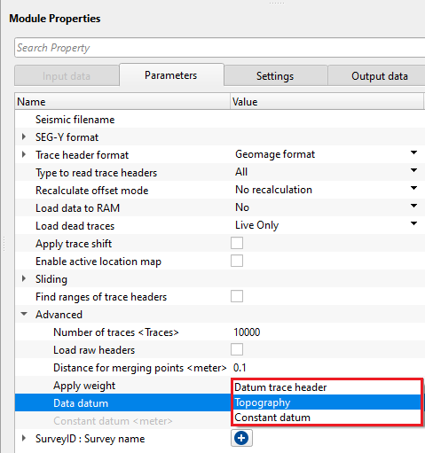
Datum trace header - it takes the datum values from the input trace headers
Topography - reads the input data from the topography level
Constant datum - assigns a constant datum value to the input trace headers. Specify a constant datum value.
Constant datum - specify the constant datum value.
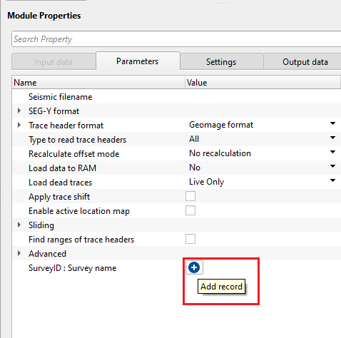
SurveyID : Survey name - it helps to assign survey ID and survey name to the input data which helps later in the processing to identify different surveys by using the survey ID or survey name parameters.
To add a Survey ID, click on ![]() and it will add Survey ID & Survey name fields.
and it will add Survey ID & Survey name fields.
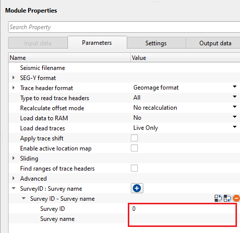
Survey ID - specify Survey ID. It should be an integer number.
Survey name - specify Survey name
![]()
![]()
Number of threads - One less than total no of nodes/threads to execute a job in multi-thread mode. Limit number of threads on main machine.
Skip - By default, FALSE(Unchecked). This option helps to bypass the module from the workflow.
![]()
![]()
Output DataItem - this generates the output data items that will be used as a reference/connection for the next modules which are going to be used in the workflow.
Output SEG-Y data handle - generates the Output SEG-Y data handle that will be used as a connection/reference to Input SEG-Y data handle.
Output trace headers - generates Output trace headers that can be set as a reference to Input trace headers.
Output gather - generates Output gather if the Load data to RAM is YES. In that case, this can be set as reference to Input gather.
Output stack line - generates output stack line.
Output crooked line - generates crooked line
Output bin grid - outputs output bin grid.
Output sorted headers - outputs default sorted headers however these sorted headers can't be used as a sorted headers.
Output raw Trace headers - outputs raw/original trace headers which ignores all the trace header modifications, calculate offsets, ignoring/muting dead traces etc.
Table Text Header - outputs the table text header as a vista item for visual QC.
Table Binary Header - outputs binary header as a vista item. This table can be exported by using "Export table" module.
Sample interval - displays input data sample interval
Data length - displays input data record length
Trace vector size - displays total number of input traces
Raw trace vector size - displays total number of raw traces
Number of sources - displays total number of shot points
Number of receivers - displays total number of receivers. By default, -1
Number of CMP - displays total number of bin/cdp/cmp. For raw field SEG-Y data without any geometry, this will be -1.
Number of dead traces - displays total number of dead traces if the load dead traces option was chosen as Dead only.
Number of live traces - displays total number of live traces.
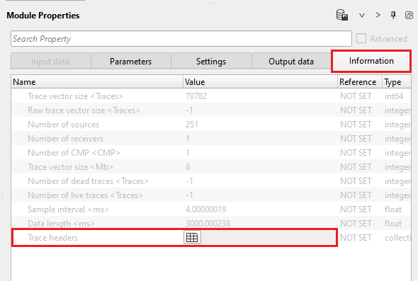
Trace headers - this displays all the trace headers information if the user selects the option "Find trace header range".
![]()
![]()
In this example section, we are covering various topics which are NOT essentially related to Read SEG-Y traces but they are common to all the modules in g-Platform.
How to display gathers using Enable active location map & Load data to RAM?
Enable active location map:
This option allows the user to display the content of the SEG-Y files. After reading the input SEG-Y and setting up all the parameters including Enable active location map as TRUE (Checked), execute Read SEG-Y traces module and launch Vista items by right click on Read SEG-Y traces module.
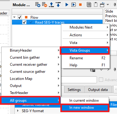
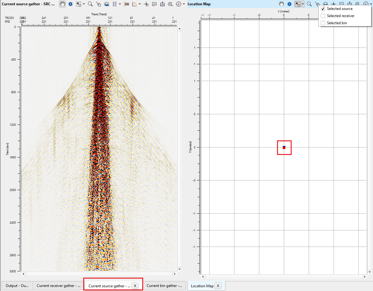
On the location map, go to Set control item icon ![]() and select "Selected source", Selected receiver & Selected bin. You can select all of them or only one. You may observe that the location map is blank (since there are no coordinates available in the trace headers). Click anywhere on the location map and it will display Selected source/receiver/bin in their respective windows(Current source gather/receiver gather/bin gather).
and select "Selected source", Selected receiver & Selected bin. You can select all of them or only one. You may observe that the location map is blank (since there are no coordinates available in the trace headers). Click anywhere on the location map and it will display Selected source/receiver/bin in their respective windows(Current source gather/receiver gather/bin gather).
To go through all gathers of the input data, use the action item menu and slide through the entire line or go to previous or next gather by using the Hot keys.
Load data to RAM:
If this box is checked, the program will load all of the traces to RAM memory. Traces loaded to RAM can be used as a gather input for modules that normally would be used in the Seismic loop module. Traces can also be displayed by the module. However, only do this if the data set is small enough to fit in the RAM memory of your system. We recommend NOT to use this option for large dataset(s). This will lead to run out of system memory which eventually freezes g-Navigator session.
Output will be displayed in Output gather window.
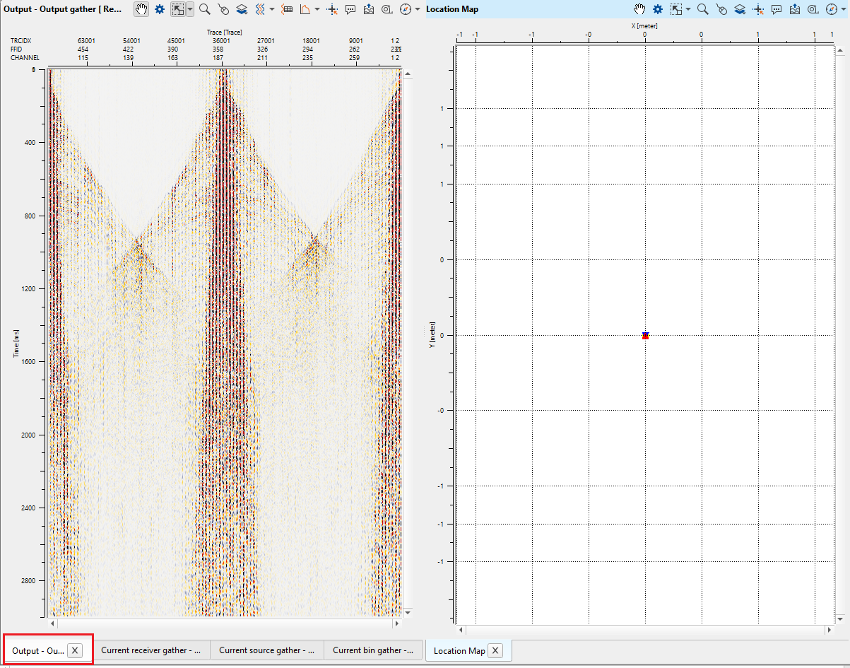
To view the gathers, use Magnifying (Zoom) icon or place the mouse(hand symbol will appear) either on horizontal axis or vertical axis and scroll up/down of the mouse wheel. Alternatively, hold Ctrl+MB1 and draw inside the Output gather window to zoom the data.
To view/edit the display parameters, there are various icons available in each window. These icons may be more/less for each window but their primary task remains the same.
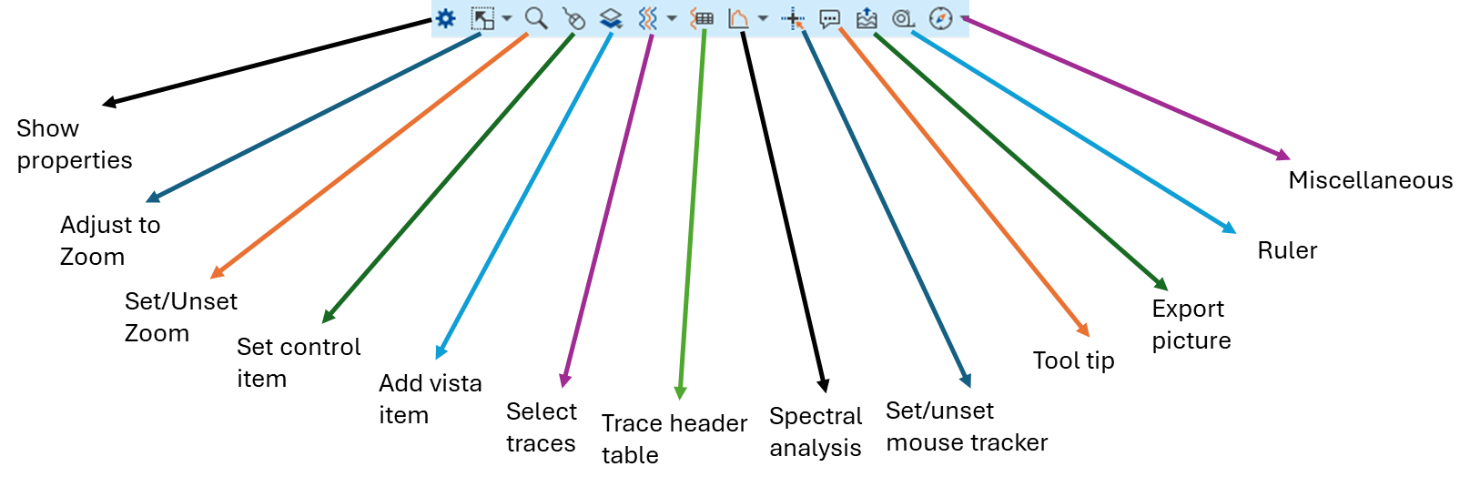
How to annotate trace headers, change display (wiggle mode/density), trace header information, spectral analysis etc?
Trace annotation: To add trace headers to the input display, click on ![]() icon, it will open View Properties window. This has two tabs. View & Vista.
icon, it will open View Properties window. This has two tabs. View & Vista.
View - it has the information related to horizontal/vertical scaling, color bars, trace header annotations etc.
Vista(s) - it is divided into two parts. Vista item, Vista item properties.
To make any changes, the user first select the Vista item. Then the corresponding Vista item properties will appear below.
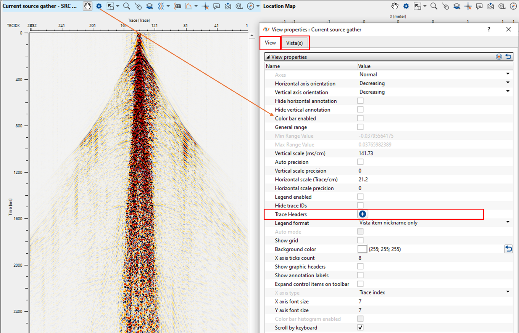
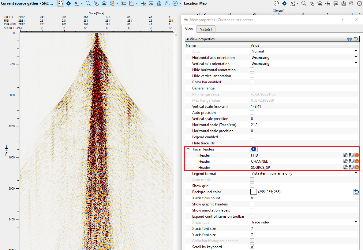
Click on ![]() icon. It will add a row with trace header. If the user wants more trace headers, add as many trace headers as they want by clicking
icon. It will add a row with trace header. If the user wants more trace headers, add as many trace headers as they want by clicking ![]() icon multiple times.
icon multiple times.
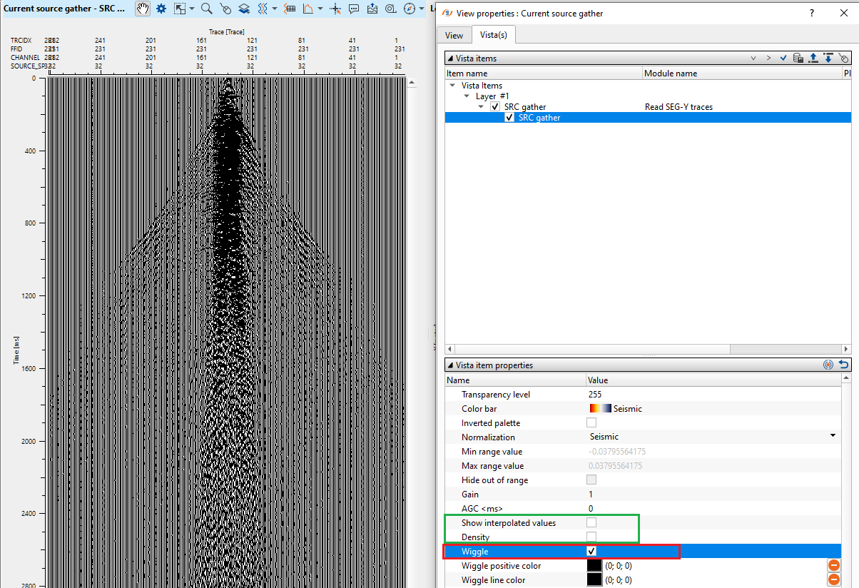
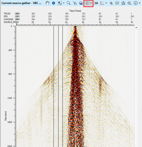
Change Display:
To change the display from density to wiggle mode or vice versa, go to Vista(s) tab of View properties window
•Select SRC gather or any Vista item and go to Vista view properties.
•Go to Color bar and choose the desired color bar from the available option from the menu.
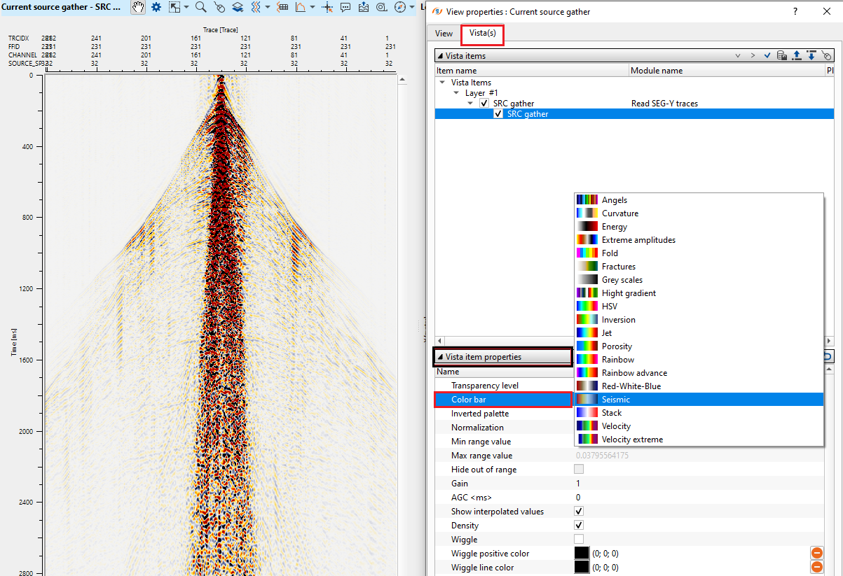
Similarly, to change the display from Density to Wiggle mode, Uncheck Show interpolated values & Density and Check Wiggle option.
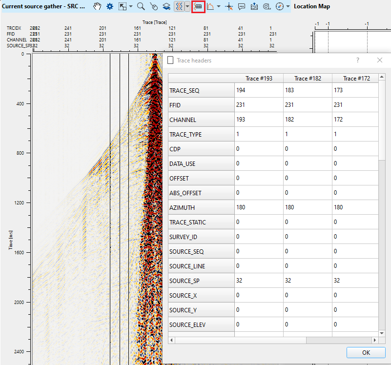
Trace header information:
To know the trace header information of the Current shot gather, click on Select trace icon ![]() (upon clicking this icon, it will be activated).
(upon clicking this icon, it will be activated).
Select any trace randomly on the shot gather. A black vertical line appears on the shot gather.
Now click on Trace header table icon ![]() . It will pop-up a window with the selected trace header information.
. It will pop-up a window with the selected trace header information.
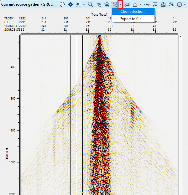
To remove the selected traces, hold MB3 and move the mouse from right to left. It will deselect the traces. Alternatively, there is an option in Select traces icon ![]() . Click on the triangle. It gives an option to clear selection. Likewise, the user can export the selected traces to file by using "Export to file" option.
. Click on the triangle. It gives an option to clear selection. Likewise, the user can export the selected traces to file by using "Export to file" option.
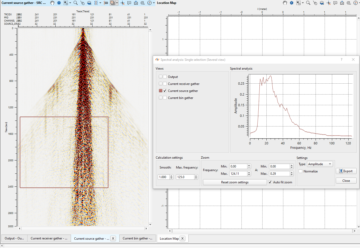
Spectral Analysis:
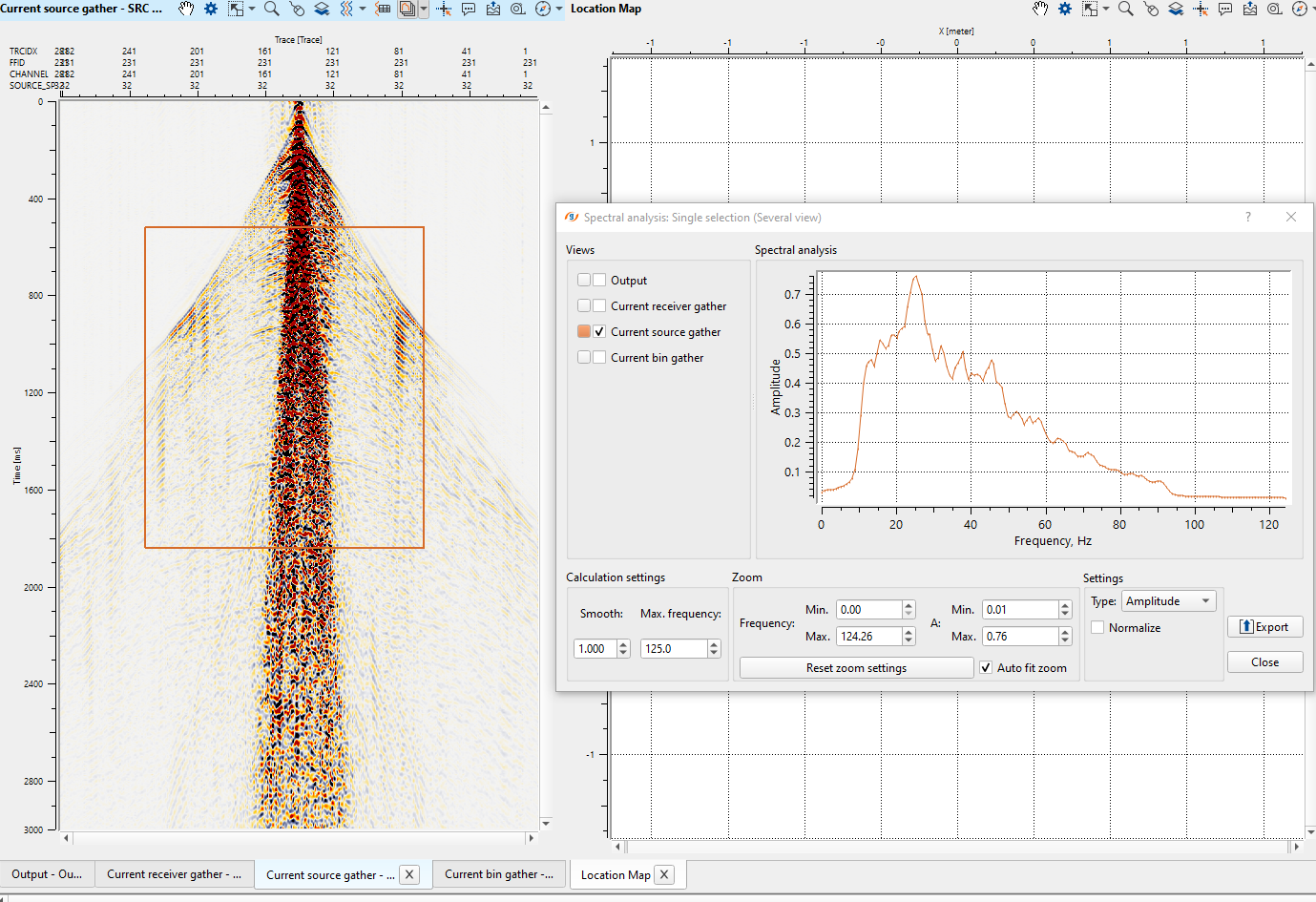
To perform spectral analysis of the input data, click on Spectral analysis icon ![]() . By default, it will perform spectral analysis for the whole window on display. If the user wants to perform the analysis of a particular area, it can be done by holding left mouse button or MB1 and draw a polygon (rectangle/square). Now it will display the spectral analysis of that particular area.
. By default, it will perform spectral analysis for the whole window on display. If the user wants to perform the analysis of a particular area, it can be done by holding left mouse button or MB1 and draw a polygon (rectangle/square). Now it will display the spectral analysis of that particular area.
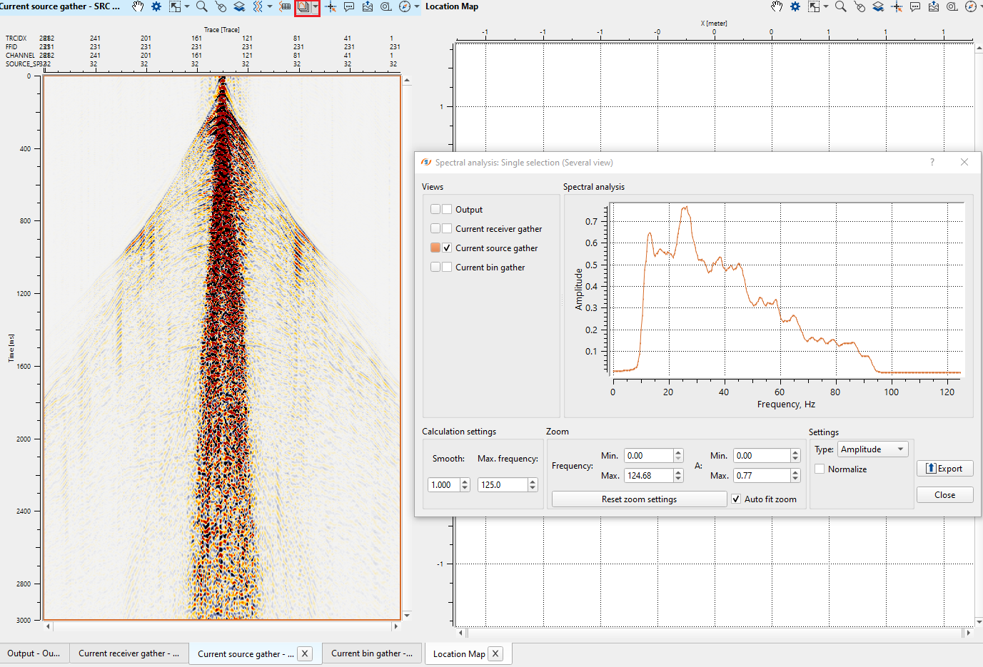
To perform spectral analysis at different times/areas, click on small triangle next to Spectral analysis icon ![]() . It gives two options, Multiple selection (Single view), Single selection (Several view).
. It gives two options, Multiple selection (Single view), Single selection (Several view).
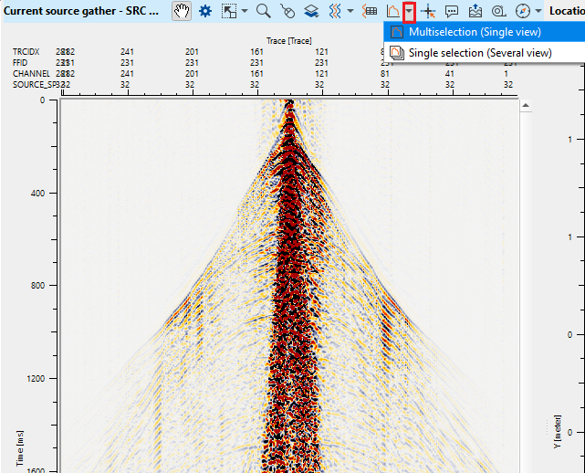
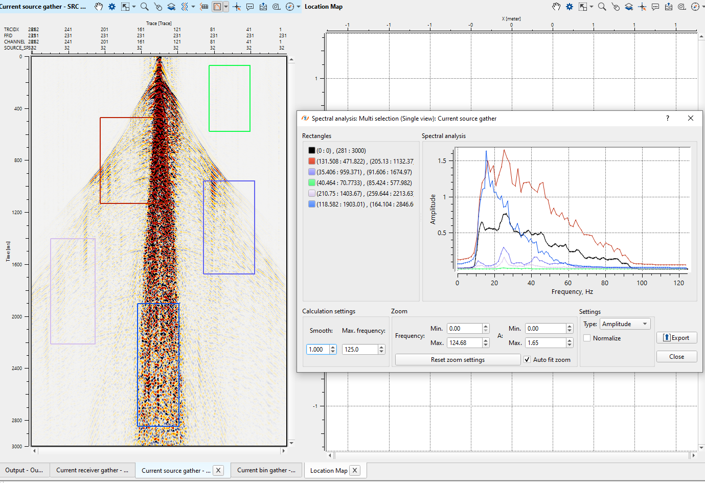
Multi selection - In this option, the user can analyze different areas for spectral response. All the areas will be displayed with different colors within the gather as well as on the spectral analysis window.
Single selection - this will analyze only one area/window and the corresponding spectral display will appear. This is the default spectral analysis option.
![]()
![]()
Slide - slides/move the input data by gather. Depending on the slide size and delay time, the gathers will animate continuously until it is stopped by.
Previous bin - moves to the previous. Hot key Ctrl+Up
Next bin - moves to the next Bin. Hot key Ctrl+Down
Previous src - moves to the previous Source. Hot key Ctrl+left arrow key
Next src - moves to the next Source. Hot key Ctrl+right arrow key
Previous rcv - moves to the previous Receiver. Hot key Alt+left arrow key
Next rcv - moves to the next Receiver. Hot key Alt+right arrow key.
![]()
![]()
YouTube video lesson, click here to open [VIDEO IN PROCESS...]
![]()
![]()
Yilmaz. O., 1987, Seismic data processing: Society of Exploration Geophysicist
 * * * If you have any questions, please send an e-mail to: support@geomage.com * * *
![]()