Attenuating reverberations, multiples using Predictive Deconvolution
Description
When the seismic sources are fired in the field (onshore/offshore), the energy travels through the sub-surface of the Earth. During the process it loses the energy. Seismic source transmits the energy through the Earth and the Earth acts as a filter.
Predictive Deconvolution compresses the seismic wavelet and suppresses reverberations and short-period multiples that are generated by layered near-surface sequences or water-bottom reflections. The module operates trace-by-trace and is based on the statistical assumption that the reflectivity series is random and the wavelet is minimum-phase. The predictive deconvolution operators are calculated and applied using a Wiener-Levinson algorithm, which solves for the least-squares inverse filter within each time window defined by the user.
This module performs trace by trace predictive minimum phase deconvolution. Deconvolution analysis windows are designed within the module. The predictive deconvolution operators are calculated and applied using a Wiener-Levinson algorithm. This algorithm
Multiple time windows (called Horizons) can be defined simultaneously, each with its own operator length, predictive interval, and noise level. This allows time-variant deconvolution, where different deconvolution parameters are applied in different time zones of the record. The Horizons parameters control the computation in each analysis window, and the taper parameter blends results smoothly at zone boundaries.
Note: This module is deprecated. For new workflows, consider using the Spike Decon or Decon Gabor modules.
Input DataItem
Connect the seismic gather to be deconvolved. The module accepts pre-stack gathers (shot gathers, CMP gathers, or offset gathers) or post-stack sections in the time domain. Each trace in the gather is processed independently, trace by trace. The input gather must be in the time domain.
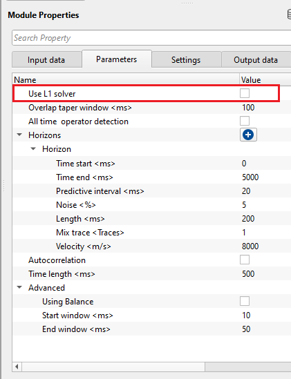
Parameters
All deconvolution windows and operator settings are configured here. At least one Horizon entry must be defined before the module can execute.
Overlap taper window
Sets the length of the cosine taper (in seconds) applied at the boundary between adjacent Horizon time windows. Default: 0.10 s. When multiple Horizons are defined, the deconvolution output from each zone is blended with its neighbour over this taper length to avoid abrupt amplitude discontinuities at zone boundaries. Increase this value if you observe step-like amplitude jumps between zones in the output.
All time operator detection
When enabled, the autocorrelation used to estimate the deconvolution operator is computed over the full trace length rather than only within the Horizon's Start Time to End Time window. Default: off. Enable this option when the time window defined in a Horizon is too short to produce a stable autocorrelation estimate, for example in very shallow target zones.
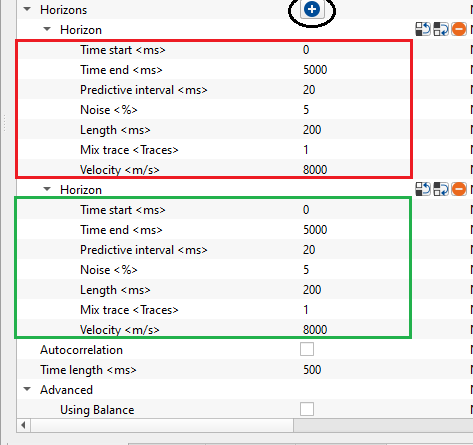
Horizons
The Horizons collection defines one or more time-variant deconvolution windows. Each entry in the collection specifies an independent analysis zone with its own deconvolution parameters. Add one Horizon per distinct time zone in the data where different deconvolution settings are needed. Horizons must not overlap in time, and Start Time must be less than End Time.
Time start
The start time of the deconvolution analysis window for this Horizon, in seconds. Default: 0 s. This is typically set to the beginning of the seismic record or to the onset of the target reflection zone. The autocorrelation for operator estimation is computed within the Time start to Time end window, so it should span a representative portion of the wavelet train to be suppressed.
Time end
The end time of the deconvolution analysis window for this Horizon, in seconds. Default: 5 s. Must be greater than Time start. The window between Time start and Time end provides the data from which the autocorrelation function is estimated. A wider window yields a more stable operator estimate but may average over time-variant wavelet changes.
Predictive interval
The prediction lag distance of the deconvolution operator, in seconds. Default: 0.02 s (20 ms). This is the key parameter for controlling what the deconvolution suppresses. Set the predictive interval equal to the two-way travel time of the multiple to be removed. For example, to suppress water-bottom multiples with a period of 80 ms, set this value to 0.08 s. A value of zero or very small value approximates spike (spiking) deconvolution, which compresses the wavelet maximally. The predictive interval must be smaller than both the operator Length and the window duration (Time end minus Time start).
Noise
The pre-whitening (noise damping) level added to the autocorrelation zero-lag before solving the Wiener-Levinson equations, expressed as a fraction of the zero-lag value. Default: 0.05 (5%). Pre-whitening stabilises the matrix inversion and prevents the operator from boosting noise. Use higher values (0.1–0.3) on noisier data or in zones with poor signal-to-noise ratio; use lower values (0.01–0.03) on clean, high-quality data where maximum wavelet compression is desired. Increasing the noise level will reduce the aggressiveness of the deconvolution.
Length
The length of the deconvolution operator, in seconds. Default: 0.2 s (200 ms). The operator length must be greater than or equal to the Predictive interval. A longer operator is better at capturing and inverting a complex wavelet or at suppressing long-period multiples, but it requires a proportionally wider analysis window to estimate stably. A rule of thumb is to set the length to at least three times the dominant wavelet period. The length must be less than the analysis window (Time end minus Time start).
Mix trace
The number of adjacent traces over which the autocorrelation function is averaged before computing the deconvolution operator. Default: 1 (no mixing). Setting this value to 1 means the operator is computed and applied independently for each trace. Increasing this value to 3 or 5 averages the autocorrelation over a small ensemble of neighbouring traces, which can stabilise the operator estimate on noisy data or data with strong amplitude variations between traces. Use values of 3–7 for noisy pre-stack gathers; keep at 1 for post-stack data where trace-to-trace amplitude differences are meaningful.
Velocity
The mute velocity used to define the NMO-corrected first-arrival mute for the analysis window within this Horizon, in m/s. Default: 8000 m/s. This parameter excludes refracted first arrivals and muted regions from the deconvolution operator estimation. Setting a very high velocity (e.g., 8000 m/s) effectively disables the mute and uses the full trace for estimation. For shot-domain processing where direct arrivals and refractions should be excluded, set this to the approximate first-arrival velocity of the near-surface.
Autocorrelation (QC Output)
When the Autocorrelation option is enabled, the module computes the autocorrelation of the input and output gathers and makes them available as separate data items for visual QC. This is useful for verifying that the deconvolution has successfully whitened the spectrum and collapsed the wavelet.
Autocorrelation
Enables computation of the autocorrelation gather for both the input and output data. Default: off. When enabled, two additional output gathers (Autocorrelation input and Autocorrelation output) become available in the module's output view. Comparing these before and after autocorrelations confirms the degree of wavelet compression achieved by the deconvolution. Enable this during parameter testing to verify that the operator is effectively whitening the spectrum.
Time length
The operator length used when computing the autocorrelation QC gathers, in seconds. Default: 0.5 s. This controls the lag window over which the autocorrelation function is evaluated. A larger value captures longer-period correlations and is useful for detecting long-period multiples, while a smaller value focuses on the immediate wavelet shape. This parameter is active only when Autocorrelation is enabled.
L1 Solver (Advanced)
The L1 solver group provides an alternative iterative deconvolution approach based on sparse (L1-norm) optimisation rather than the standard least-squares (L2-norm) Wiener-Levinson solution. The L1 solver produces sparser reflectivity estimates and is more robust to non-Gaussian noise and isolated large-amplitude events (spikes). By default the standard Wiener-Levinson solver is used.
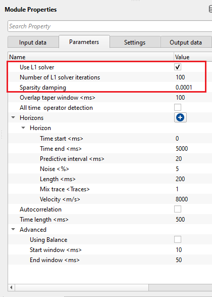
Use L1 solver
Activates the iterative L1 sparse deconvolution solver in place of the standard Wiener-Levinson algorithm. Default: off. When enabled, the Number of L1 solver iterations and Sparsity damping parameters become visible. Use the L1 solver when data contain impulsive noise or when a sparser-than-minimum-phase reflectivity model is desired. Processing with the L1 solver is slower than the default algorithm.
Number of L1 solver iterations
The maximum number of iterations for the L1 sparse optimisation solver. Default: 100; minimum: 1. More iterations allow the solver to converge more fully to the sparse solution but increase processing time. For most data, 50–100 iterations are sufficient. This parameter is visible only when Use L1 solver is enabled.
Sparsity damping
A small regularisation constant (epsilon) that controls the transition between L1 and L2 behaviour in the iteratively reweighted least-squares optimisation. Default: 0.0001; minimum: 1e-9. Smaller values enforce stronger sparsity (fewer, larger reflectors) but can make the solver less stable. Larger values (e.g., 0.01) make the solution smoother and closer to the L2 minimum. This parameter is visible only when Use L1 solver is enabled.
Advanced
The Advanced group provides optional amplitude pre-conditioning before the deconvolution operator is applied. This is useful when traces have strongly varying amplitude levels that would otherwise bias the autocorrelation estimate.
Using Balance
Applies a trace balance (amplitude normalisation) to the input gather before computing the deconvolution operator. Default: off. When enabled, each trace is normalised within the balance window (Start window to End window) before the deconvolution operator is estimated. After deconvolution the amplitude scaling is restored by dividing back by the balance factors. This produces operators that are less sensitive to traces with anomalously high or low amplitudes. Enable when processing data with strong near-offset to far-offset amplitude variation, or data with significant geometric spreading differences between traces.
Start window
The start time of the window used for the balance amplitude normalisation, in seconds. Default: 0.01 s. This parameter is active only when Using Balance is enabled. Set this to exclude any strong first-arrival energy that would dominate the balance computation.
End window
The end time of the window used for the balance amplitude normalisation, in seconds. Default: 0.05 s. This parameter is active only when Using Balance is enabled. Ensure this window covers a sufficient portion of the trace to produce a stable amplitude estimate.
Settings
The Settings section controls how the module handles bad or not-a-number (NaN) values found on input traces, and how execution is distributed across threads. The module supports multi-threaded processing for improved performance on large datasets.
Notify - It will notify the issue if there are any bad values or NaN. This is halt the workflow execution.
Fix - It will fix the bad values and continue executing the workflow.
Continue - This option will continue the execution of the workflow however if there are any bad values or NaN, it won't fix it.
For most production workflows, select Fix to automatically zero out any bad values and continue processing without interruption. Select Notify during QC runs when you want to be alerted to data quality issues before committing to a full processing pass.
Output DataItem
The deconvolved seismic gather. Each trace has been processed by the Wiener-Levinson predictive deconvolution operator computed within the analysis windows defined by the Horizons. The output is in the time domain with the same trace geometry and sample interval as the input. Connect this to subsequent processing modules such as band-pass filtering or stacking.
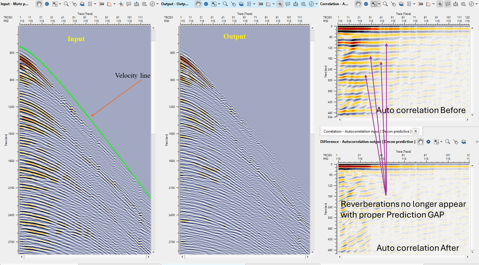
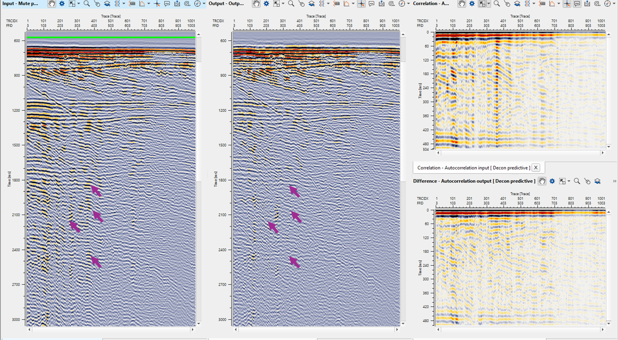
Two additional outputs are available when Autocorrelation is enabled: Autocorrelation input shows the autocorrelation of the original data and Autocorrelation output shows the autocorrelation of the deconvolved data. The output autocorrelation should show a narrower, more spike-like central lobe compared to the input, confirming successful wavelet compression.
This modules doesn't have any information available so the user can ignore it.
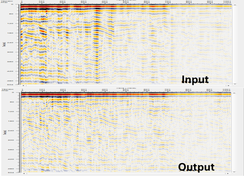
Examples
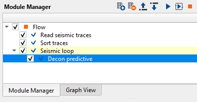
The figures below illustrate the Decon predictive module interface and typical before/after results.
Action Items
This modules doesn't have any action items so the user can ignore it.
References
Robinson, E. A. and Treitel, S., 1980, Geophysical Signal Analysis: Prentice-Hall.
![]()
![]()
Yilmaz. O., 1987, Seismic data processing: Society of Exploration Geophysicist