Random noise attenuation using FX Decon filter
![]()
![]()
FX Decon filter module is designed for random noise attenuation. Data from T-X (Time - Space) domain is converted to F-X (Frequency-Space) domain using Fourier transformation along the time axis. A predictive deconvolution filter operator is calculated and used in T-X domain window for coherent impulse selection. This Decon prediction filter is applied to the data by working on each trace by trace with each frequency slice.
FX Decon predictive filter is useful in attenuating the random, incoherent noise. It is also used to attenuate the multiples since the multiples are predictable with their predictability where the primaries won't have the spatial predictability.
![]()
![]()
Input DataItem
Input gather - FX Decon filter should be used on cmp gather or post-stack gather to attenuate any random, incoherent noise. Connect/reference to output gather.
Connect this input to the output of the preceding module in the workflow — for example, the output of a stacking module, NMO correction, or any other processing step that produces a seismic gather. The FX-Decon filter is most effective on data that already has good spatial sampling (regular trace spacing with minimal gaps). Applying it to sparsely sampled or geometrically irregular data may produce artefacts rather than noise attenuation.
![]()
![]()
Horizontal sliding window - specify the number of traces should be used in designing the prediction filter. These traces are moved in sliding order based on the user defined parameters. Minimum horizontal sliding window should be 5. Shorter horizontal window is useful where the prediction is localized. With higher/longer horizontal window, it improves the frequency resolution however smears the data especially the dipping events. Depending on the geological setup, choose the appropriate parameters.
The default value is 10 traces. The minimum allowed value is 5 traces. A typical starting point for marine or land post-stack data is 10–20 traces. Use a shorter window (5–10 traces) in areas with steeply dipping reflectors or lateral velocity variation to preserve structural detail. Use a longer window (20–40 traces) on flat, laterally continuous data where higher frequency resolution is beneficial. Note that the window must always be larger than the Number of filter points parameter.
Number point for filter design - specify the total number of coefficients required to design the prediction filter. The longer the prediction filter points, the better suppression of the noise however it may distort the primary signal. Number of filter points should be less than that of horizontal sliding window.
The default value is 4 filter points. The minimum allowed value is 1. This parameter must always be strictly less than the Horizontal sliding window size — the module will report an error if this condition is violated. A value of 4 is appropriate for most applications. Increasing this value (e.g., to 6–8) can improve noise suppression on heavily contaminated data, but risks attenuating signal energy. Keep this value small relative to the sliding window to maintain a well-conditioned prediction filter.
Time window - within the user defined time window, deconvolution filter applied spatially to the input data. Specify the time window. Minimum time window should be 200 ms. Recommended shorter time window.
The default value is 0.5 s (500 ms). The minimum allowed value is 0.2 s (200 ms). The filter operator is redesigned independently for each overlapping sub-window along the time axis, allowing the filter to adapt to non-stationary noise and varying frequency content with depth. Shorter time windows (200–300 ms) give better adaptation to rapidly changing noise character but may reduce statistical stability. Longer windows (500–1000 ms) are more statistically robust but less adaptive. For most post-stack applications a value of 0.5 s is a good starting point.
Taper window - taper parameter is essential to avoid any edge effects/sharp boundary when applying the deconvolution prediction filter within the user defined and time and horizontal sliding window parameters.
The default value is 0.1 s (100 ms). The minimum allowed value is 0 s (no taper). A cosine taper of this length is applied at the beginning and end of each time window before the prediction filter is computed and applied, blending adjacent windows together smoothly. Setting this value to zero removes edge-effect protection and may introduce amplitude discontinuities at window boundaries. Increasing the taper beyond 0.1 s provides additional blending at the cost of slightly reduced effective window length.
Min frequency - specify minimum frequency that should be considered
The default value is 1 Hz. The minimum allowed value is 0 Hz. Frequency components below this threshold are excluded from the prediction filter design and are passed through unmodified to the output. Set this value to match the low-frequency limit of the usable signal bandwidth — typically 3–8 Hz for land data and 1–5 Hz for marine data. Very low frequencies often have poor signal-to-noise ratio and may cause filter instability if included.
Max frequency - specify maximum frequency that should be considered
The default value is 80 Hz. The minimum allowed value is 0 Hz. Frequency components above this threshold are excluded from the prediction filter design and are passed through unmodified to the output. Set this value to match the high-frequency limit of the usable signal bandwidth — typically the Nyquist frequency minus a safety margin (e.g., 120 Hz for 250 Hz Nyquist data). Extending the maximum frequency too close to Nyquist may introduce aliasing artifacts into the filtered output.
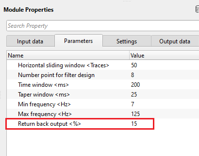
Return back output - this allows the user to choose how much percentage of original data should be added/mixed back to the filtered data after applying FX Decon filter. Specify the % of input data should be mixed back.
The default value is 0 (0%). The valid range is 0.0 to 1.0 (representing 0% to 100%). At the default of 0, the output is the fully filtered gather with no mixing. At 1.0 (100%), the output is identical to the input with no noise attenuation applied. Intermediate values blend the filtered and original data: for example, setting this to 0.15 adds 15% of the original data back into the filtered result, which can help recover any signal energy that was inadvertently attenuated. This parameter is useful when the filter is applied aggressively and some signal protection is needed.
![]()
![]()
Auto-connection - By default, TRUE(Checked).It will automatically connects to the next module. To avoid auto-connect, the user should uncheck this option.
Bad data values option { Fix, Notify, Continue } - This is applicable whenever there is a bad value or NaN (Not a Number) in the data. By default, Notify. While testing, it is good to opt as Notify option. Once we understand the root cause of it,the user can either choose the option Fix or Continue. In this way, the job won't stop/fail during the production.
Notify - It will notify the issue if there are any bad values or NaN. This is halt the workflow execution.
Fix - It will fix the bad values and continue executing the workflow.
Continue - This option will continue the execution of the workflow however if there are any bad values or NaN, it won't fix it.
Calculate difference - This option creates the difference display gather between input and output gathers. By default Unchecked. To create a difference, check the option.
When enabled, the module computes and outputs an additional Gather of difference (input minus output). Enable this option during parameter testing to visually verify that the filter is removing noise rather than signal. Disable it in production processing to reduce memory usage and processing time.
Number of threads - One less than total no of nodes/threads to execute a job in multi-thread mode. Limit number of threads on main machine.
This module supports multi-threaded execution. Set this value to the number of CPU cores you wish to dedicate to the module. Setting it too high on a shared machine can degrade overall system performance — a common practice is to use the total number of available cores minus one, leaving one core free for the operating system and other workflow modules.
Skip - By default, FALSE(Unchecked). This option helps to bypass the module from the workflow.
When Skip is enabled, the module passes the input gather through to the output without applying any filtering. This is useful for A/B testing — enable Skip to compare the unfiltered result against the filtered result without removing the module from the workflow.
![]()
![]()
Output DataItem
Output gather - generates the FX Decon filter applied output gather. This can be used as an external output or connect/reference to any other module.
The output gather has the same dimensions (number of traces and number of samples) as the input gather. Random, incoherent noise has been suppressed by the predictive deconvolution filter in the F-X domain. Connect this output to subsequent modules such as migration, attribute extraction, or display. The output can also be saved directly to a SEG-Y file as an intermediate QC result.
Gather of difference - generates the difference gather before and after application of FX Decon filter.
This output is only produced when the Calculate difference option is enabled in the Settings section. The difference gather represents the noise component removed from the data (input minus output). Inspecting this gather is the recommended way to QC the filter — it should contain primarily incoherent noise and should show no coherent reflector energy, which would indicate over-filtering and signal leakage into the noise estimate.
There is no information available for this module so the user can ignore it.
![]()
![]()
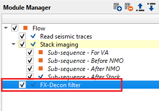
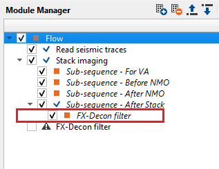
In this example workflow, we apply FX Decon filter on a post stack gather to attenuate the random noise. FX Decon filter can be added within the Stack Imaging - sub-sequence after stack or outside the Stack Imaging.
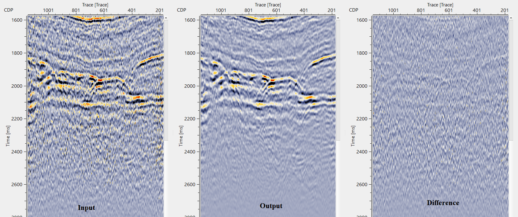
The above image is created using below parameters. 15% of original data is mixed back.
![]()
![]()
There are no action items available for this module so the user can ignore it.
![]()
![]()
YouTube video lesson, click here to open [VIDEO IN PROCESS...]
![]()
![]()
Yilmaz. O., 1987, Seismic data processing: Society of Exploration Geophysicist
 * * * If you have any questions, please send an e-mail to: support@geomage.com * * *