FXY Deconvolution filter for 3D dataset
![]()
![]()
FXY Decon Filter is designed to attenuate random noise by prediction of the non-random signal content in a seismic trace.
Apply the FX Deconvolution Filter (FXY in case of 3D) prior to minimum or zero phase deconvolution to get the better results. This should give a cleaner operator design leaving the output less contaminated by random noise. Each input trace is transformed from T-X (Time-Space) domain into the F-X (Frequency-Space) domain. Groups of traces are used to design filters to predict the Fourier components of adjacent traces. The number of traces used to design the filter.
Provide number of traces (Horizontal sliding window) from T-X domain to frequency domain. Now in the frequency domain, for each frequency (Frequency range Minimum and Maximum) it generates a complex Wiener Filter to predict the amplitude and phase of the next trace. Likewise it predicts the amplitude and phase for the next adjacent traces and so on. This process is carried out in forward and reverse direction and the output sample for this frequency is the average of the forward and reverse predictions. Finally predicted traces are reconstructed in the frequency domain and then transformed back into the time domain.
![]()
![]()
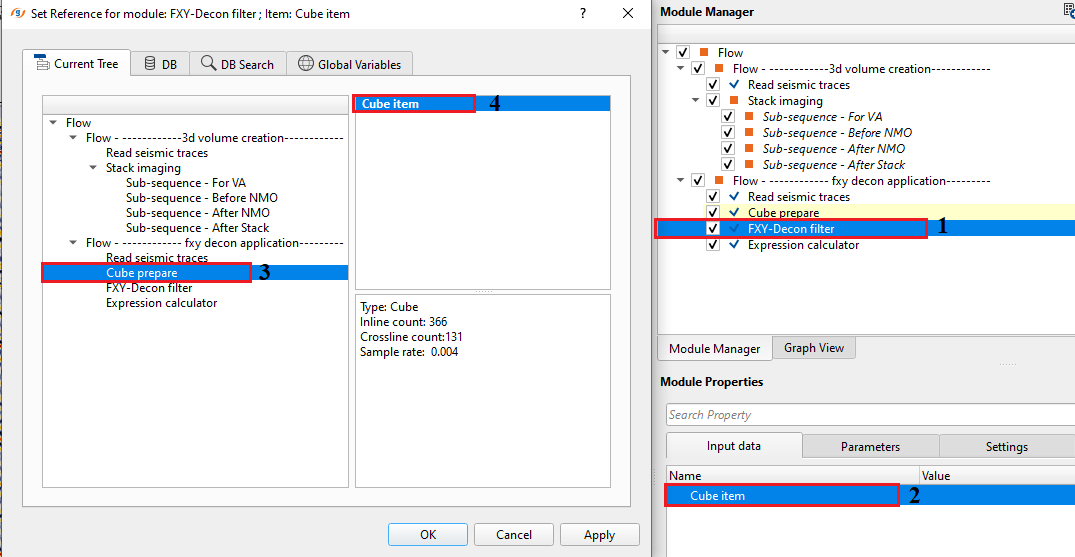
Cube item - connect/reference to the input 3D volume item to perform FXY Deconvolution. More detailed explain about cube item is explained in the Example section.
The Cube item is a mandatory input that provides the 3D seismic volume on which the FXY deconvolution filter will be applied. It must be created beforehand using the Cube prepare module, which loads the volume into memory. Unlike the standard FX Decon filter (which operates trace-by-trace inside a sub-sequence), FXY Decon requires the full 3D cube to be resident in RAM so that it can apply the prediction filter across both the inline and crossline directions. Connect this item to the output of a Cube prepare module. See the Example section below for step-by-step instructions on how to set up the workflow.
![]()
![]()
Horizontal sliding window - specify the number of traces should be used in designing the prediction filter. These traces are moved in sliding order based on the user defined parameters. Minimum horizontal sliding window should be 5. Shorter horizontal window is useful where the prediction is localized. With higher/longer horizontal window, it improves the frequency resolution however smears the data especially the dipping events. Depending on the geological setup, choose the appropriate parameters.
Default: 10 traces. Minimum: 5 traces. This parameter controls the spatial extent of the prediction operator in the inline or crossline direction. A window of 10 traces is a practical starting point for most datasets. Use smaller values (5–7) when the geology has strong lateral heterogeneity or steeply dipping reflectors, because a larger window will mix energy from structurally different areas and smear the output. Use larger values (15–20) when the data is relatively flat-lying and structurally simple, as this improves the signal-to-noise ratio of the Wiener filter design. Note that the Number point for filter design must always be smaller than this value.
Number point for filter design - specify the total number of coefficients required to design the prediction filter. The longer the prediction filter points, the better suppression of the noise however it may distort the primary signal. Number of filter points should be less than that of horizontal sliding window.
Default: 4. Minimum: 1. This value must be strictly less than the Horizontal sliding window; the module will report an error if this condition is violated. A typical ratio is 3:1 to 4:1 between the window and the filter length (for example, 10 traces window with 4 filter points). Increasing this value makes the Wiener filter more adaptive and capable of suppressing complex noise patterns, but at the risk of over-fitting and signal leakage. If you observe that coherent reflectors are being attenuated along with the noise, reduce this value.
Time window - within the user defined time window, deconvolution filter applied spatially to the input data. Specify the time window. Minimum time window should be 200 ms. Recommended shorter time window.
Default: 0.5 s (500 ms). Minimum: 0.2 s (200 ms). The filter is applied independently within overlapping time windows of this length. Shorter windows allow the filter to adapt to time-varying noise characteristics (for example, where noise levels change rapidly with depth), but windows that are too short may not contain enough data for robust Wiener filter estimation. Longer windows are more stable statistically but assume that the noise is stationary across the window. A value of 0.5 s is suitable for most production runs; reduce to 0.3 s or less when you need strong time-variant noise suppression in shallow versus deep sections.
Taper window - taper parameter is essential to avoid any edge effects/sharp boundary when applying the deconvolution prediction filter within the user defined and time and horizontal sliding window parameters.
Default: 0.1 s (100 ms). Minimum: 0 s. At the edges of each time window and at the boundaries of the horizontal sliding window, a cosine taper of this length is applied to blend the filtered output smoothly with its surroundings. This prevents abrupt amplitude steps or ringing artifacts at window boundaries. A value of 0.1 s is adequate for most data. Set to 0 only if you are certain the data has no edge effects; otherwise keep it at least 50–100 ms. Increasing the taper beyond 0.2 s will reduce the effective processing area and may not improve results.
Min frequency - specify minimum frequency that should be considered
Default: 1 Hz. Minimum: 0 Hz. The Wiener prediction filter is only designed and applied for frequencies above this threshold. Very low frequencies (below 5 Hz) are often dominated by ground-roll energy or acquisition noise rather than random noise, so excluding them by setting Min frequency to 5–8 Hz can improve the filter's effectiveness on the target signal band. Set to 0 only if you need the filter to act across the entire spectrum from DC upward.
Max frequency - specify maximum frequency that should be considered
Default: 80 Hz. Minimum: 0 Hz. The filter is not applied to frequencies above this value. Set this to roughly the highest frequency at which coherent signal is present in your data (typically 60–100 Hz for typical seismic surveys). Applying the prediction filter beyond the signal bandwidth offers no noise-reduction benefit and may introduce artifacts, so match this value to the effective bandwidth of your data as determined from a frequency spectrum analysis. The combination of Min frequency and Max frequency defines the pass-band over which the Wiener predictor operates.
Return back output - this allows the user to choose how much percentage of original data should be added/mixed back to the filtered data after applying FX Decon filter. Specify the % of input data should be mixed back. By default, 0.
Default: 0 (0%). Range: 0 to 1 (0% to 100%). After the FXY filter is applied, the output for each sample is computed as: Output = Filtered + Factor × (Original − Filtered). At 0 (the default), the output is the fully filtered result. At 1.0, the module returns the original unprocessed data unchanged. Intermediate values blend the filtered and original signals, acting as a mild noise-attenuation control. Use values of 0.1–0.3 when you wish to preserve some of the original amplitude character while still reducing random noise. This is particularly useful when the data contains weak but geologically meaningful lateral amplitude variations that you do not want the filter to over-smooth.
Apply on selected inline/crossline - this section deals with application of FXY Decon filter operation on selected inline/crosslines or the entire volume. During the testing phase, the user should select any particular/target inline or crossline to fine tune the FXY Decon filter parameters. After finalizing the parameters, it can be executed on the entire volume.
This container groups the three sub-parameters that control whether the filter is applied to the entire 3D volume or only to a single test inline and/or crossline. Use the Selected inline/crossline toggle to enable single-line testing mode. In testing mode, the Vista outputs (Inline output, Inline input, Inline difference, Crossline) are populated with just the selected lines so you can inspect the effect of the parameters quickly before committing to a full volume run. Once you are satisfied with the results, disable this option and execute on the whole cube — the Whole data Vista output is only populated during a full-volume run.
Selected inline/crossline - choose the inline and/or cross line of the input volume. By default, FALSE
Default: false. When set to true, the module operates only on the inline and/or crossline numbers specified in the Inline and Crossline parameters below, enabling rapid QC of filter settings on a representative line before running the full volume. Enable this for parameter testing and disable it for production processing.
Inline - specify the inline number to perform FXY Decon filter operation. By default, -1 which means it considers all inlines within the volume.
Default: -1 (process all inlines). Active only when Selected inline/crossline is set to true. Enter the actual inline number from your survey geometry (for example, 200) to restrict processing to that single line and view the result in the Inline output Vista. Set to -1 when you want to process the entire volume.
Crossline - specify the cross line number. By default, -1 which means all crosslines within the volume.
Default: -1 (process all crosslines). Active only when Selected inline/crossline is set to true. Enter the actual crossline number from your survey (for example, 79) to restrict testing to that line and view the result in the Crossline Vista. You can specify both an inline and a crossline simultaneously to QC the filter in both directions at once before running the full volume.
![]()
![]()
Distributed execution - if enabled: calculation is on coalition server (distribution mode/parallel calculations).
Bulk size - chunk size is RAM in megabytes that is required for each machine on the server (find this information in the Information, also need to click on action menu button for getting this statistics)
Limit number of threads on nodes - limit numbers of of threads on nodes for performing calculations.
Job suffix - add a job suffix
Set custom affinity - an axillary option to set user defined affinity if necessary.
Set custom affinity - true - If checked, provide the affinity name.
Affinity - add your affinity to recognize you workflow in the server QC interface.
Number of threads - One less than total no of nodes/threads to execute a job in multi-thread mode. Limit number of threads on main machine.
Run scripts - it is possible to use user's scripts for execution any additional commands before and after workflow execution
Script before run - path to ssh file and its name that will be executed before workflow calculation. For example, it can be a script that switch on and switch off remote server nodes (on Cloud).
Script after run - path to ssh file and its name that will be executed before workflow calculation.
Skip - By default, FALSE(Unchecked). This option helps to bypass the module from the workflow
![]()
![]()
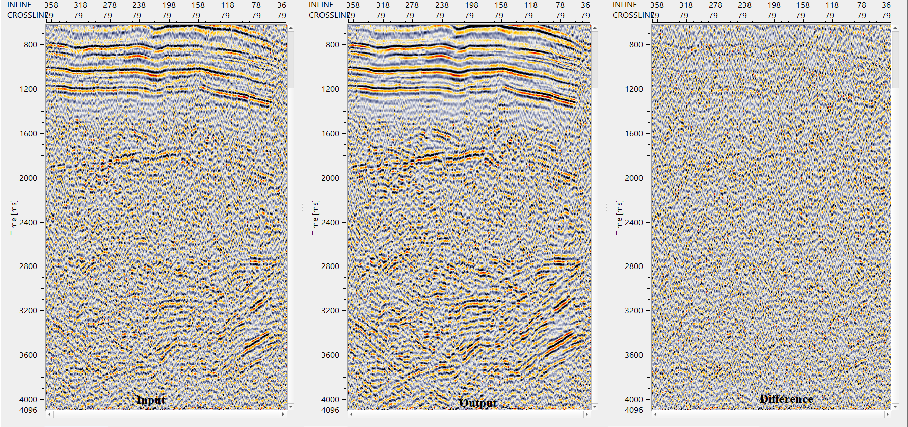
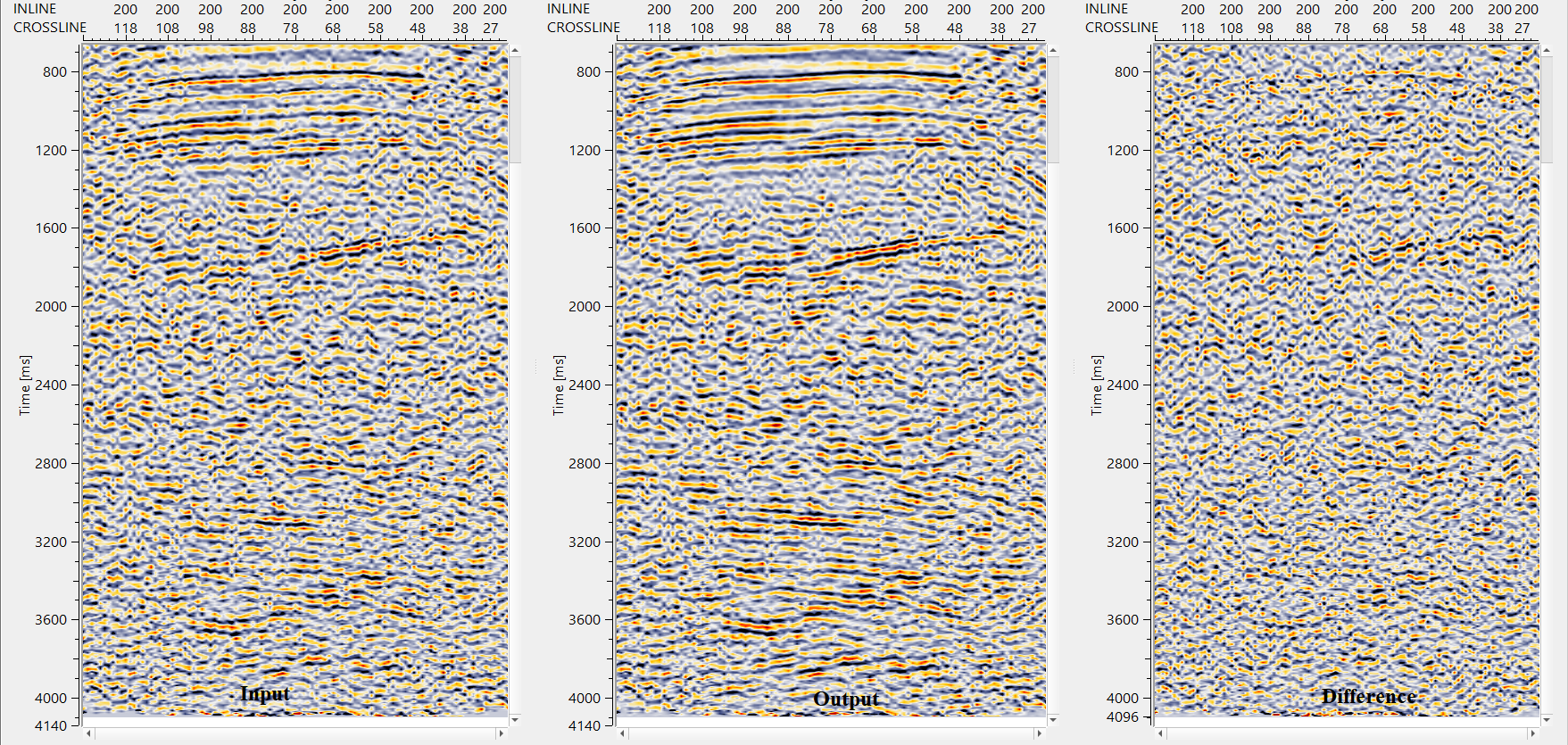
Inline output - generates the FXY Decon filter applied inline output gather as a vista.
Available only in Selected inline/crossline mode. Displays the noise-attenuated inline section after the FXY Deconvolution filter has been applied. Use this Vista to confirm that random noise has been reduced and that coherent reflectors are preserved. Compare side by side with Inline input and Inline difference for parameter tuning.
Inline input - generates the input inline as a vista
Available only in Selected inline/crossline mode. Displays the unprocessed original inline section taken directly from the Cube item. Use this as the reference image when evaluating the noise attenuation achieved in the Inline output Vista.
Inline difference - generates the difference gather of inline before and after application of FXY Decon filter.
Available only in Selected inline/crossline mode. Shows the sample-by-sample difference (Output minus Input) for the selected inline. This Vista represents the noise component that has been removed by the filter. Inspect it to verify that the removed signal is dominated by random noise and does not contain coherent events such as reflection wavelets. If you see organised reflector-like energy in the difference, the filter is too aggressive — reduce Number point for filter design or widen the Horizontal sliding window.
Crossline - generates the FXY Decon filter applied cross line output gather as a vista.
Available only in Selected inline/crossline mode. Displays the filtered crossline section for the crossline number specified in the Crossline parameter. Inspecting both the Inline output and this Crossline Vista in testing mode allows you to confirm that the filter performs consistently in both spatial directions before committing to a full-volume run.
Whole data - generates FXY Decon filter applied full volume
Available only in full-volume mode (when Selected inline/crossline is false). After the filter is applied to all inlines and crosslines of the 3D cube, the entire processed volume is merged and made available through this Vista item. This is the primary output for production use. The Inline output, Inline input, Inline difference, and Crossline Vistas are not populated in this mode.
There is no information available for this module so the user can ignore it.
![]()
![]()
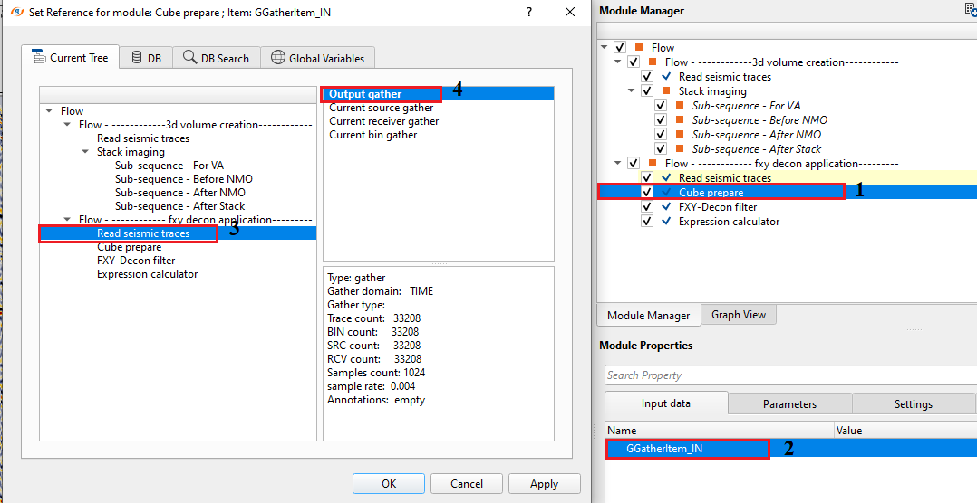
In this example, apply FXY Decon filter on a 3D cube. Unlike FX Decon filter, where it can be added inside the sub-sequence process of Stack Imaging or any other procedure, FXY Deon filter works on a "Cube item". Input for this module should be a Cube item.
How to create/generate Cube item?
If there is an existing 3d volume, then
•Read the volume by using "Read seismic traces" and choose option Load data to RAM as YES.
•Add "Cube prepare" module and connect/reference to Output gather of "Read seismic traces". This will create the cube item.
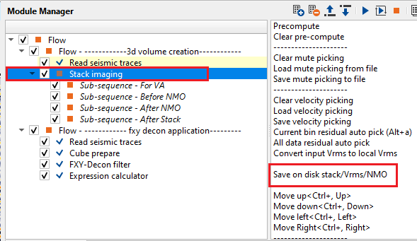
In case there isn't any 3d volume, then how to create a 3D volume?
•Read input seismic traces using "Read seismic traces" module.
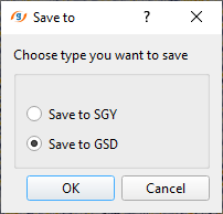
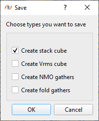
•Inside the "Stack Imaging" module, go to action items and select "Save on disk stack/Vrms/NMO" option. Select "save to GSD" option and select "Create stack cube". Give it a name and it will create the 3D volume for the entire survey.
•follow the same procedure as explained above when there is an existing 3D volume to create cube item.
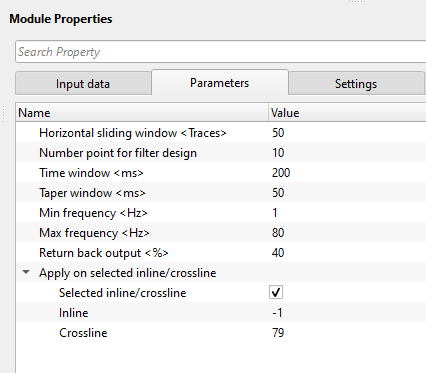
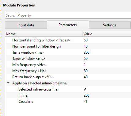
Now, select the desired Inline and/or Crossline and adjust the parameters as per the data requirement. Execute the module and generate the Vista items for QC. For this exercise, crossline 79 & inline 200 is selected. Below parameters showing for Cross line 79 & Inline 200.
![]()
![]()
This module has no custom action buttons. All processing is triggered by the standard Execute command in the workflow. Use the Selected inline/crossline parameters in the Parameters tab to control whether you are running in QC mode (single line) or production mode (full volume).
![]()
![]()
YouTube video lesson, click here to open [VIDEO IN PROCESS...]
![]()
![]()
Yilmaz. O., 1987, Seismic data processing: Society of Exploration Geophysicist
 * * * If you have any questions, please send an e-mail to: support@geomage.com * * *