Description
This module processes raw, uncorrelated Vibroseis seismic records by cross-correlating each input trace with the Vibroseis sweep signal. The cross-correlation collapses the long swept-frequency pulse train produced by the Vibroseis source into a compact, impulsive wavelet — the Klauder wavelet — making the correlated record directly comparable to data acquired with conventional impulsive sources such as dynamite.
The sweep signal can be supplied as an external wavelet gather (the recommended approach when the recorded pilot sweep is available) or extracted directly from the first trace of the input gather when no external sweep is provided. After cross-correlation, an optional spectral deconvolution step can be applied to whiten the spectrum and convert the zero-phase Klauder wavelet toward minimum phase, which is required by many standard deconvolution workflows.
In addition to the correlated output gather, the module saves several diagnostic wavelets — the modeled sweep, the sweep autocorrelation, the minimum-phase wavelet, and the Vibroseis deconvolution operator — allowing the user to inspect and quality-control each step of the conversion. Use this module as the first processing step whenever Vibroseis raw field records are imported into a project.
Cross-Correlation background:
Cross-Correlation is a measure of similarity of two series f (t)and g (t)as a function of the displacement of one relative to the other.
Let us consider two real functions {\displaystyle f}f and g{\displaystyle g} differing only by an unknown shift along the X-axis. By doing the cross-correlation, we can find how much {\displaystyle g}g must be shifted along the X-axis to make it identical to {\displaystyle f}f . The formula essentially slides the {\displaystyle g}g function along the X-axis, calculating the integral of their product at each position. When the functions match, the value of {\displaystyle (f\star g)}( fx g ) is maximized. This is because when peaks are aligned, they make a large contribution to the integral. Similarly, when troughs align, they also make a positive contribution to the integral because the product of two negative numbers is positive.
The cross-correlation of functions f( t) and g( t) is equivalent to the convolution of f *(− t) and g( t).
{\displaystyle f\star g=f^{*}(-t)*g.} f x g= f* (- t) * g ; where f* denotes the complex conjugate of f
Vibroseis Data Conversion:
Vibroseis source is a long train of sine waves of increasing or decreasing frequencies. Conventional impulsive source like dynamite produces a single discrete impulse for each event, whereas the Vibroseis source will show the event as a pulse train. In an uncorrelated seismic record, the pulse trains for each event overlap and cannot be separated by the human eye. However, after cross-correlation with the input sweep, each event should appear as a synthetic pulse which has the shape of the auto-correlation of the sweep.
Following are the advantages …
1.Since we know the form of the source signal, we can easily remove the back ground noise from the data using the source signal
2.We know the Vibroseis sweep frequency band, anything outside the frequency band limit of the sweep can be considered as a noise and that can be filtered out.
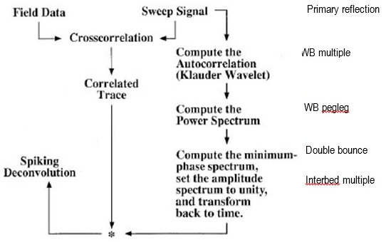
Figure 1. Schematic diagram of Vibroseis data Cross Correlation and Deconvolution (Image courtesy: SEG Wiki)
Input data
Input DataItem
The primary seismic dataset containing raw, uncorrelated Vibroseis field records. Each trace in this dataset holds the uncorrelated response of the earth convolved with the Vibroseis sweep — the overlapping pulse trains that must be collapsed by cross-correlation. Connect this input to the raw field data imported directly from SEG-Y or the project database before any other processing is applied.
Input gather
The seismic gather to be processed in the current iteration. This input is populated automatically as the module steps through the dataset gather by gather. Each gather is cross-correlated with the sweep signal and, if deconvolution is enabled, the resulting correlated gather is further processed to whiten the spectrum.
Input sweep
An optional external sweep wavelet gather used as the reference signal for cross-correlation. Connect a recorded pilot sweep or a synthetic sweep generated by the Create sweep module here. When this input is connected, the module resamples the supplied sweep to match the input data sample interval before performing cross-correlation. If this input is left unconnected, the first trace of the input gather is used as the sweep — this is appropriate only when the sweep signal has already been recorded as the leading trace of each record.
Parameters
Execute deconvolution
When set to True, spectral deconvolution is applied after cross-correlation to whiten the amplitude spectrum and suppress the sweep autocorrelation side-lobes. This moves the correlated wavelet toward minimum phase and is required as a precursor to conventional spiking or predictive deconvolution steps. The default value is False — cross-correlation alone is performed and the output retains its zero-phase Klauder wavelet character.
Vibroseis data
This parameter group controls how the sweep autocorrelation window is computed.
Cross Correlation Time
The length of the cross-correlation window in seconds, used when computing the sweep autocorrelation that is written to the diagnostic output. This value should be set equal to or slightly longer than the sweep duration used in acquisition. The default value is 5 s, which is appropriate for standard exploration sweeps of 4–6 s duration. Shorter sweeps used in shallow high-resolution surveys may require a smaller value (for example, 2–3 s).
Sweep model
This parameter group controls the trapezoidal bandpass taper applied in the frequency domain to the sweep spectrum before cross-correlation. Enabling the bandpass suppresses energy outside the sweep frequency band, effectively band-limiting both the correlated output and the noise. The four corner frequencies define the trapezoidal shape of the filter: energy below Fr1 and above Fr4 is zeroed; energy between Fr1 and Fr2 ramps linearly from zero to full amplitude; energy between Fr2 and Fr3 passes unmodified; and energy between Fr3 and Fr4 ramps back to zero.
BandPass Fr1
The low-cut frequency (Hz) below which the filter response is zero. This is the lowest corner of the trapezoidal bandpass taper. Set this value to the lowest frequency present in the sweep — frequencies below this threshold are pure noise and should be excluded. The default value is 1 Hz. This parameter is active only when Execute bandpass is enabled.
BandPass Fr2
The low-pass taper end frequency (Hz). The filter ramps linearly from zero at Fr1 to full amplitude at Fr2, creating a smooth low-frequency roll-on that avoids spectral ringing. Set this value to the start frequency of the sweep (the lowest frequency actually emitted by the Vibroseis source). The default value is 5 Hz. This parameter is active only when Execute bandpass is enabled.
BandPass Fr3
The high-pass taper start frequency (Hz). The filter passes energy at full amplitude between Fr2 and Fr3. Above Fr3 the filter begins to roll off toward zero at Fr4. Set this value to the end frequency of the sweep (the highest frequency emitted by the Vibroseis source). The default value is 125 Hz. This parameter is active only when Execute bandpass is enabled.
BandPass Fr4
The high-cut frequency (Hz) above which the filter response is zero. Energy above this frequency is treated as high-frequency noise outside the sweep band and is removed. Set this value comfortably above Fr3 — typically 1.5 to 2 times the Nyquist frequency of useful signal — to allow a gentle taper without cutting into the sweep band. The default value is 250 Hz. This parameter is active only when Execute bandpass is enabled.
Whitening factor
A stabilization noise level (expressed as a fraction of the peak spectral amplitude) added to the denominator of the cross-correlation filter to prevent division by near-zero values at frequencies where the sweep has low energy. Higher values produce a more whitened (broader bandwidth) result but reduce the fidelity of the spectral shaping. Lower values preserve more of the sweep spectrum shape but may amplify noise at frequencies where the sweep power is weak. The default value is 0.01 (1% of peak spectral power). Typical values range from 0.001 to 0.05 depending on the signal-to-noise conditions of the data.
Decon operator
This parameter group controls the design of the shaping filter that converts the correlated (zero-phase Klauder) wavelet into a minimum-phase equivalent. These parameters are active only when Execute deconvolution is set to True.
Decon Domain
Selects the domain in which the minimum-phase deconvolution operator is computed. Available options are:
Frequency (default) — the minimum-phase spectrum is derived via the cepstral method in the frequency domain. This approach is more accurate for broadband sweeps and handles non-stationary spectra better. Use this option for most Vibroseis datasets.
Time — the operator is computed using Wiener-Levinson least-squares inversion in the time domain. This can be preferable when the sweep autocorrelation is already well-behaved and a compact time-domain operator is desired.
Noise
The pre-whitening noise level (expressed as a fraction of the zero-lag autocorrelation value) added to stabilize the Wiener-Levinson inversion when computing the deconvolution operator. This parameter has the same role as the pre-whitening percentage used in standard predictive deconvolution: a value of 0.01 adds 1% white noise to the autocorrelation diagonal before solving for the operator. Increasing this value makes the operator more stable but reduces its resolving power. The default value is 0.01 (1%). This parameter is active only when Execute deconvolution is True.
Filter length
The length of the shaping (deconvolution) operator in seconds. A longer operator can model more complex wavelet shapes and produce a better minimum-phase approximation, but it also requires more computation time and may become unstable if the signal-to-noise ratio is low. The default value is 0.1 s (100 ms), which is appropriate for most exploration sweep bandwidths. For very broadband sweeps or datasets with complex sweep signatures, consider increasing this value to 150–200 ms. This parameter is active only when Execute deconvolution is True.
Output data
The module produces the correlated output gather as its primary result, plus four diagnostic wavelet datasets that can be saved for quality control and further analysis. Connect any of these outputs to a data store module in the workflow to save them to the project database.
Output gather (correlated seismic data)
The primary output gather in which each trace has been cross-correlated with the sweep signal and, if requested, spectrally deconvolved. Reflections that were spread over the full sweep duration in the raw records are now compressed into short pulses aligned at the correct two-way traveltimes, ready for standard pre-processing (geometry assignment, amplitude correction, deconvolution, stacking, and migration).
Output Vibs Decon filter
The computed shaping operator (deconvolution filter) that converts the correlated Klauder wavelet into minimum phase. Saving this output allows the user to inspect the operator length and shape, verify that the operator is stable, and apply the same operator to other datasets if required.
Min Phase Wavelet
The minimum-phase equivalent of the Klauder wavelet, derived from the sweep autocorrelation using the cepstral or Wiener-Levinson method selected by the Decon Domain parameter. This wavelet can be used for wavelet extraction, wavelet QC, or as input to subsequent deconvolution modules that require an estimate of the source wavelet.
Sweep
The modeled or recorded sweep signal as used internally by the module during cross-correlation. Saving and reviewing this output confirms that the correct sweep was loaded, the sample rate matches the data, and the amplitude spectrum of the sweep covers the expected frequency band.
Sweep autocorrelation
The autocorrelation of the sweep signal within the Cross Correlation Time window. This is the theoretical shape of the correlated wavelet (the Klauder wavelet) and is used to design the deconvolution operator. Inspect this output to verify the side-lobe level and symmetry of the Klauder wavelet before enabling deconvolution.