SRME 2D/3D

Multiple attenuation by using SRME (Surface Related Multiple Elimination/Estimation)

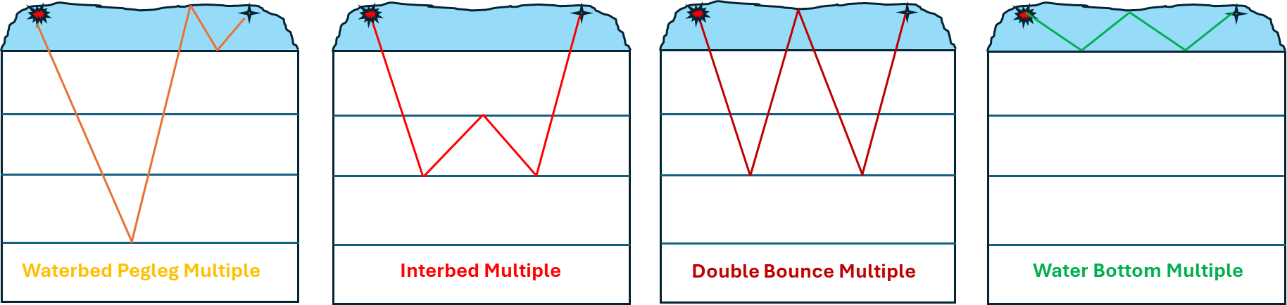
The presence of multiples in the seismic data will give a false information to the interpreters. Multiples energy is a major issue in marine seismic data processing. Multiples energy obstruct the primary energy/reflections of the sub-surface. In order to attenuate the multiples, there are various methods available. There are many kinds of multiples present in the seismic data. Water Bottom multiples, Peg Leg multiples, Interbed multiples etc.

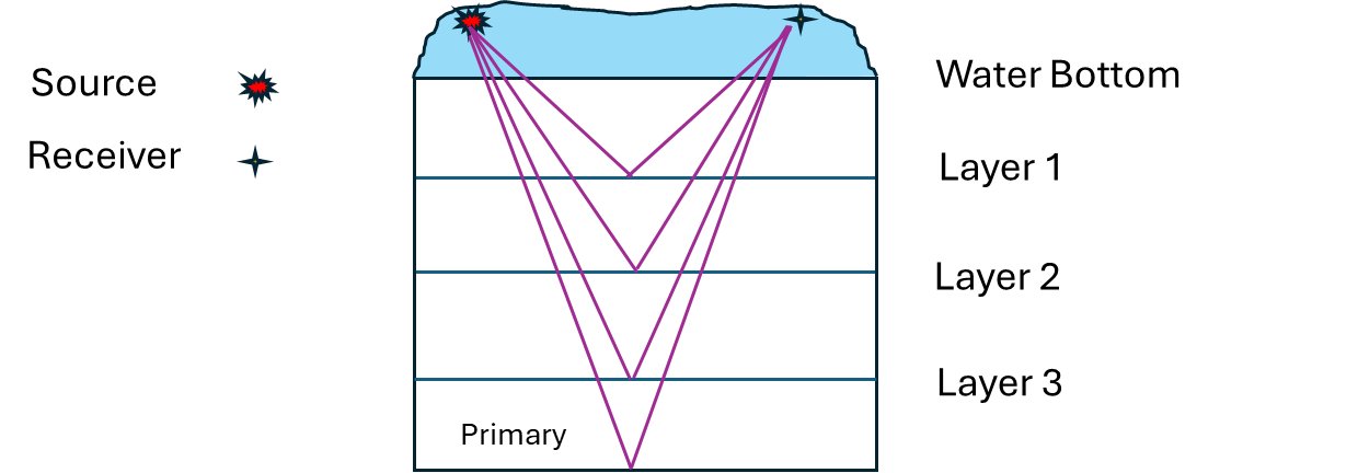
To attenuate the multiples we need an algorithm which can predict the multiples from the input data and later subtract the multiples from input to get the multiple free data. It can be achieved in different ways.

1.Periodicity based

2.Move out based

Surface related multiples are predicted using auto-convolutions of input data. The predicted multiple energy is then adaptively subtracted from the input gathers.

In g-Platform, in order to predict the multiple model, first supply the input data in correct sorting order (usually shot gather). Prepare the input data with necessary pre-conditioning like muting the data above first arrivals. This helps in multiple prediction. Also, make sure to have the source water depth values in the trace headers in case the user wants to mute the input and multiple model above the first arrivals.

How to do multiple model testing in g-Platform?

After making necessary references/connections to the SRME 2D/3D module, right click on the SRME 2D/3D module and select Vista Groups -> All Groups -> In new window. This will add "Location map, Current Input gather, Current multiple gather" windows.

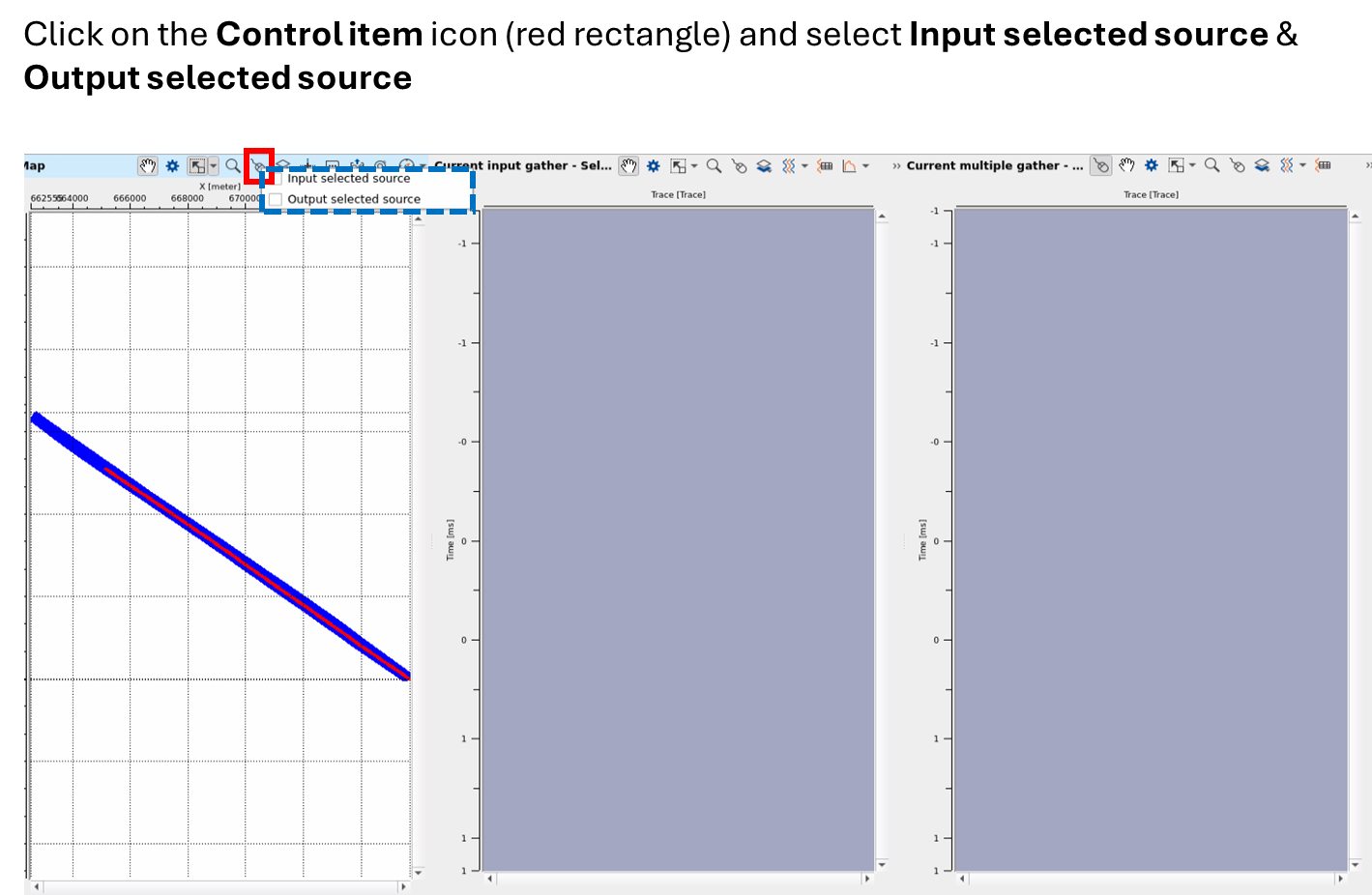
Go to Location map and select the Control item . This will opens up two options. Input selected source and Output selected sources. Check these options. This will allow to select any shot point position on the location map. For your reference, you can see in the above image.

Now Select any shot from the location map ( Preferably the shots which are not close to the start of the line)

If we click on the Show properties of the "Current Input gather" window, it will have something like

Selected gather in - This is the current input gather or the selected gather from the location map

Selected gather in with extrapolation - This is the extrapolated gather if we opt for internal extrapolation within the SRME 2D/3D module.

Selected gather in after preprocessing - This is the pre-processed gather if we choose any pre-processing like muting the data above first arrivals etc.

Selected gather out subtracted - This is the adaptively subtracted output gather. This is the final output gather.

If we want to see any one of them, we need to toggle off/uncheck the gather one above it.

Now to predict the multiple for the selected input gather, we need to go to actions items of SRME 2D/3D module which is next to Module Manager

Click the “Selected gather: calculate multiples” which gives the predicted multiple for that particular shot.

Likewise, the user can try different shot locations by selecting from the location map and try with different parameters until get the satisfactory results.  

Once the predicted multiple is satisfactory, the user can try the adaptive subtraction parameters test (though it is meant for a quick visualization QC, more robust parameter testing can be done in the later stage of "Adaptive subtraction"). To execute and see the results of the Adaptive subtraction,“Selected gather: adaptive subtraction” which can adaptively subtract the multiples and gives the multiple free data.

SEG-Y data handle - Connect/reference to Output SEGY data handle of "Read seismic traces" module.

Input trace headers (of seismic data) - Connect/reference to Output trace headers of "Read seismic traces" module.

Output trace headers - Optional.

Vrms model - Optional

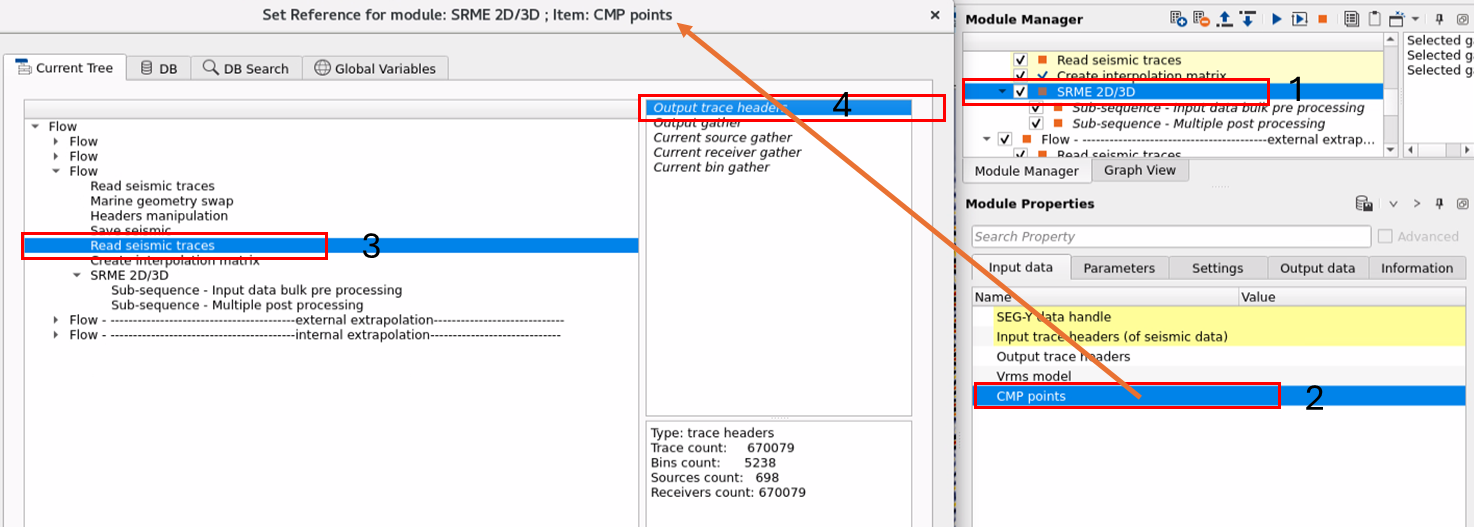
CMP points - This is optional however if the multiple model prediction is "Run by" CMP option then the user should connect the Output trace headers of the "Read seismic traces" module. From these trace headers, it will take the CMP geometry.

Output file name - Provide the output file name of the multiple model gather

Sort by { As is, Offset, Abs offset, Receiver-id offset, Receiver-id abs offset } - This parameter allows the user the sort the data in different sorting order. This will avoid any additional sorting required before the SRME 2D/3D procedure. There are various sorting options available. Choose the required one from the drop down menu.

As is - It will keep the input data as it is

Offset - Sort the data in offset mode

Abs Offset - Sorts the data in Absolute offset mode

Receiver-id offset - This sorting method sorts the data in Receiver-id and offset mode.

Receiver-id Abs offset - This option sorts the data in Receiver-id and Absolute offset mode.

Output creation type { Multiple model, Subtracted gathers } - By default, Multiple model. This parameter gives the option to choose which will be the final output from the SRME 2D/3D module.

Multiple model - This will output the predicted multiple model

Subtracted gathers - This option output the final output gather without multiples. This uses the input and predicted multiple model and subtract the multiples using adaptive subtraction parameters.

Run type { By CMP, Usual, Light } - Choose the available options to run the multiple model prediction.

By CMP - The modeling of the multiples takes place in the CMP domain. If this option is chosen then we should connect/reference the Output trace headers to CMP points in the Input data type.

Usual - This is the regular multiple prediction where it uses the usual source-receiver pairs for predicting the multiple model.

Light - This is the fastest and less accurate run type for predicting the multiple model. Even though it uses the source-receiver pairs but considers less number of source-receiver pairs in multiple model prediction. Due to this, it is fast however the resultant multiple model may not accurate.

Middle point aperture - The distance between the nearest source and receiver pair. This parameter defines the multiple collection area.

Aperture in s-line - The spatial extent of the sources along the source line. This determines the boundaries whithin which the source data can be utilized to predict and eliminate the multiples.

Aperture in r-line - The spatial extent of the receivers along the receiver line. This aperture determines the region of receiver coverage relevant to the data used in the predicting of the multiples.

Bounding width ratio (3D) - This parameter controls the area extent of the multiple prediction and elimination. It helps in controlling the source and receiver combinations are within the specified boundary limits so that the correct and accurate the model prediction can be achieved and unnecessary data is  not included in the multiple prediction procedure.

Modeling type { All combinations, SRSR } - Multiple model prediction can be done using two combinations. One is All combinations and SRSR - Source-Receiver-Source-Receiver combination.

All combinations - It Considers all possible combinations of source and receiver pairs. This will include all the primary reflections and multiple reflections of 1st order, 2nd order, 3rd order etc.

SRSR - In this method, it considers the Source-Receiver pairs. In this case, the source generates the primary reflections and transmits through various layers of the earth, reflected back to the source and receiver multiple times. This method doesn't require more computation power unlike the all combinations where the later one considers all the possible source-receiver combinations thus needs more computing power.

Pair traces max offset deviation to - This parameter is used to control how much offset between source and receiver pairs can vary but still valid for predicting the multiples. This parameter is crucial since if the offset deviation between source and receiver is too much then there are unwanted source-receiver pair traces will participate in the multiple prediction procedure. To avoid this, it is necessary to control the offset deviation between source-receiver pairs.

DRP aperture - DRP is nothing but Data Related Prediction. This is basically the boundary within which the multiples are predicted based on the source-receiver geometry. This is the actual data which is available within the seismic survey.

Use fold - By default, Unchecked. If checked this option, it will consider the fold of the data.

Move kinematics { None, To result offset, To cmp (by cmp only) } - Kinematics of the seismic waves like travel times, velocities and travel time paths are used to predict the multiples. For prediction of the multiples, we need to where the primary and secondary reflections (1st and 2nd order multiples) occur. This can be achieved by the kinematics.

None -  

To result offset - moving the kinematics to the result offset (full offset) involves the modeling of full effective offset after multiple reflections resulting in precise multiple prediction however this come with a higher computational cost.

To Cmp - This option is applicable when we use the "Run Type as By CMP only". In this option, moving the kinematics to the CMP involves the application of more generalized kinematic model based on CMP.

Near offset extrapolation

Near offset extrapolation - In case if there are any missing shots at the beginning of the line, then turn ON this option to do the interpolation for better predicting the multiple model.

Replacement velocity - Provide the near surface or replacement velocity

Interpolate each streamer - By default, Unchecked which means it will extrapolate to only one streamer/cable however if this option is "Checked", it will extrapolate the near offsets for each streamer.

Maximum distance to extrapolation - Define the maximum distance for interpolation which is related to near offset interpolation

Step to extrapolate - Define the interpolation step size. Usually the receive interval or shot point interval.

Frequency parameters - Specify the frequency range of the input data that needs to be considered in multiple model prediction procedure

Min frequency - provide the minimum frequency value to be considered for the multiple model prediction.

Max frequency - provide the maximum frequency value to be considered for the multiple model prediction.

Processing FFT - It transforms the data from time domain to frequency domain using Fast Forward Transformation. Once the seismic data is transformed into frequency domain, it will be easier to distinguish primaries and multiples since multiples have distinct frequency characteristics.

Freq-amp recovery - This parameter takes care of the frequency and amplitude recovery. If the predicted multiples frequency and amplitudes are not matching then it will try to recovery both of them.

Freq-amp recovery norm - This parameter normalizes the amplitudes of the seismic signals across different frequencies. This parameter ensures that the predicted multiples and the observed (input data) should match with the frequency and amplitudes.

Sigma - threshold used to determine the reliability of the multiple model prediction.

Mute type { None, Water depth, Horizon velocity model } - Select the type of mute is used to predict the multiples from the drop down menu. Depending on the selection , the user should provide the respective input information.

For example, if the Mute type is selected as "Horizon velocity model" then they should provide the horizon information in the Multiple type input section.

None - There will be any mute applied

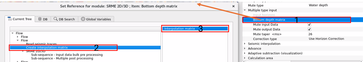
Water Depth: Multiple model prediction based on Source Water Depth values. When this option is selected, then the user should provide the Bottom depth matrix. This is referenced to "Create Interpolation Matrix" module

Horizon Velocity Model: You can pick the water bottom horizon using the SRMP module and provide the horizon information here. When the Mute type is Horizon velocity model, make sure to select the Correction type as "Use Horizon Correction" if necessary.

Multiple type input -

Input horizons - In case the Mute type is chosen as "Horizon velocity model" then we should provide the horizon.

Bottom depth matrix - Connect to the Source Water Depth values. It can be created by using Create Interpolation Matrix module. Provide the depth matrix if the multiple type as "Water depth"

Mute input Data - By Default True. It’s advised to check the input data if you select this option as "True" to make sure no primary data is muted.

Mute output Data - By Default True. It’s advised to check the Output data.

Mute taper - Provide the mute taper value to apply the mute the gather above provided taper value.

Correction type { Use Horizon Correction, NONE } -

Seismic interpolation

Interpolate input traces - Prior to model prediction, user can able to interpolate the input traces. By default it is set as False but user can select this option to interpolate the data with an appropriate regularization scheme.

Trace multiplication factor - Define the trace interpolation (multiplication factor). For example, if shot interval is 25 m and receiver interval is 12.5 m and we want to interpolate every shot to make the shot interval is same as receiver interval to predict the multiple model more accurate.

Number of iterations - Define how many iterations are required to interpolate the input traces. Remember the more number of iterations the more run time it takes. 10 no of iterations is a good starting point.

Regularization type { First derivative, Laplasian, FK, Radon } - Choose the regularization type from the available options. By default Laplasian.

We have 4 types of regularization in case if we have any missing traces or shots. Choose the appropriate one for the data regularization among the given one.

1. First derivative - This represents the rate of change of the seismic signal. This type of regularization is very useful for smoothing of the data by reducing the high frequency noise and improving the continuity of the data. In this regularization method, if a seismic trace is missing, the first derivative of the surrounding traces help estimate the missing values by looking into the change of the signal.

Weight of time derivative - this captures the rate of changes of the seismic data/wave with respect to time. If the weight of the time derivative is too high, it will over smooth the regularization of the temporal changes of the seismic data. That will leads to not to able to see the significant events like reflections and sharp transitions in the signal.

On the other side, if the weight of the time derivative is too small, it will not proper smooth the data and leaves the high frequency noise which results in poor regularization.

Weight of line derivative - this parameters captures the rate of changes of the seismic data/wave in the spatial direction. This will show how the trace is changing from one trace to the next trace spatially. This parameter controls the how strongly the regularization emphasizes the smooth variations along the spatial direction.

If the weight of is too high, it will impact the subtle features like fractures and faults in the spatial direction. In case the weight is too low, the regularization is not smooth enough which results in leaving all the high frequency noise with irregularities.

2. Laplasian - Laplasian regularization is used when the seismic data is sparse. It will helps in smoothing the data and reducing the high frequency noise especially in irregular data types.

Weight of Laplasian - this is a regularization parameter which is optimized to achieve the smoothness of the accuracy of the data by maintaining a good balance between these. Higher weight value may over smooth and this is useful when the data is too noisy. On the other side, lower weight value may not fit the model perfectly however it is useful in the case of subtle variations in the data.  

3. FK - Frequency (F) & Wavenumber (K) regularization method is useful when there is a missing seismic trace. This will transform the data from the time domain to frequency domain.

Velocity mute - define the velocity value that will suppress/mute the multiples that are associated within this velocity.

4. Radon - This regularization scheme helps in regularizing by isolating coherent features in the data such as events travel along the specific trajectory. By applying Radon regularization scheme, we can smooth the data along the specific paths and reduce the noise that are not following these paths.

P min - specify the minimum value of the ray parameter or slowness. If this value is too low, we may include low noise signals. If it is too high, we may exclude the shallow events.

P max - specify the maximum value of ray parameter of slowness. If Pmax is too high, we may include the higher distant multiples and if it is too low, we may miss the deep subsurface events.

Delta P - specify the ray parameter or slowness interval value. If the Delta P value is low, it will give a detailed information however computationally it is expensive and takes longer times. On the other side, if the Delta P value is high it reduces the computing time but the information is less in detail.

Advance

Percent padding - provide the % padding applied before and/or after regularization.

Clip big values - If any noisy/spiky/big amplitude traces are there, then it will clip or limit the amplitudes of those traces

Clip big values of amplitude - Deletes allocated high-amplitude spikes that differs from the average value in the trace in percent

Saving mode { append, direct } - Specify the mode of saving the data.

Precompute distances - By default, Unchecked. If it is checked, it will precompute the distance.

Adaptive subtraction (visualization)

Horizontal window - Total number of seismic traces are participating the adaptation window. Pay attention to number of traces. More number of seismic traces may give good understanding of the spatial variability of the seismic signal however this may not work well  in all cases we want finer details. Also, this may increase the computation time.

Vertical window - Provide the time in milliseconds

Min vertical shift - Define the smallest or minimum vertical shift of the data during the filtering process. Usually the seismic data starts from time 0 ms. We can specify this time as a minimum vertical shift. Otherwise, we can define the next available time sample. It will depend on the sample interval of the input data. If the input data is 2ms sample interval then we can put this minimum vertical shift as 2ms. In case it is 4ms then we input this value as 4ms. So, the filtering process will start from 4ms time sample onwards.

Max vertical shift - Specify the maximum vertical shift of the data during the filtering process.

Step vertical shift - Specify the step size of the vertical shift. This step size is usually of sample interval size.

Subtraction type { SVD, Cholesky, Lsqr } - There are 3 subtraction types are available. The user should select any one of them from the drop down menu and provide the parameters accordingly.

SVD - Singular Vector Decomposition: This method in adaptive subtraction works by decomposing the seismic data matrix into singular vectors and values, then separating the primary signal (high-rank components) from unwanted noise or multiples (low-rank components). By removing or filtering out the low-rank components and reconstructing the data, SVD helps to enhance the primary signal while suppressing multiples or noise.

Cholesky - Cholesky Decomposition: In the Cholesky subtraction method, the primary idea is to use the Cholesky decomposition of the auto-correlation matrix of seismic data to model and subtract multiples from the observed data. The method leverages the correlation structure between seismic traces to isolate and remove these unwanted noise/multiples, thus enhancing the clarity of the primary reflections for further interpretation.

Lsqr - Least Square method is an adaptive filtering technique used to estimate and subtract unwanted signals such as multiples or noise. It involves solving a least squares optimization problem to find the best-fit unwanted signal model, which is then subtracted from the observed data to recover the primary seismic signal. The method is flexible, data-driven, and effective for removing complex unwanted components, but it can be computationally demanding and dependent on the quality of the input data.

Lamda - This is a regularization parameters where it is used to control the balance between fitting the data and suppressing the noise/multiple data.

When the estimated multiples are less sensitive to the small variations, a large Lambda value gives more weight to the regularization term which leads to smoother solution. Whereas in the case of lesser Lambda value, the estimated multiples are closely fitted/matched with the input data however this will increase the noise levels also.

Calculation area

Calculation area mode { by sequence number, by inLine/xLine } - The restriction of data to process

Allow re calculate

First inline number(-1 no limit) - By default, -1 which means it considers all. Otherwise, specify the 1st inline number

Last inline number(-1 no limit) - By default, -1 which means it considers all. Otherwise, specify the last inline number

First crossline number(-1 no limit) - By default, -1 which means it considers all. Otherwise, specify the 1st crossline number

Last crossline number(-1 no limit) - By default, -1 which means it considers all. Otherwise, specify the last crossline number

First number(-1 no limit) - By default, -1 which means it considers all. Otherwise, specify the 1st sequence number

Last number(-1 no limit) - By default, -1 which means it considers all. Otherwise, specify the last sequence number

RND debug - By default, Unchecked. This is for R&D debugging and there is no significance in the parameter testing

Max fold - provide the maximum fold of the input data

Adaptive on processed - By default, unchecked.

SegyCacheParams -

Execute on { CPU, GPU } - select which type of processor will be used for calculations: CPU or GPU.

Distributed execution - if enabled: calculation is on coalition server (distribution mode/parallel calculations).

Bulk size - chunk size is RAM in megabytes that is required for each machine on the server (find this information in the Information, also need to click on action menu button for getting this statistics)

Limit number of threads on nodes - limit numbers of of threads on nodes for performing calculations.

Job suffix - add a job suffix.

Set custom affinity - an auxiliary option to set user defined affinity if necessary.

Affinity - add your affinity to recognize you workflow in the server QC interface.

Number of threads - limit number of threads on main machine.

Run scripts - it is possible to use user's scripts for execution any additional commands before and after workflow execution

Script before run - path to ssh file and its name that will be executed before workflow calculation. For example, it can be a script that switch on and switch off remote server nodes (on Cloud).

Script after run - path to ssh file and its name that will be executed before workflow calculation.

Skip - switch-off this module (do not use in the workflow).

Selected gather in - the user can save this selected input gather as an output.

Selected gather in with extrapolated offsets - this is the near offset extrapolated selected gather.

Selected gather in after preprocessing - any pre-processing applied on the selected input/extrapolated gather like mute, agc, band pass etc can be saved as an output gather.

Selected gather multiples - this modules outputs the selected multiple gather.

Selected gather out substracted - this is the final subtracted multiple free gather. This is also one of the outputs generated by this module.

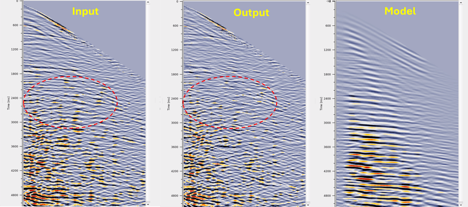
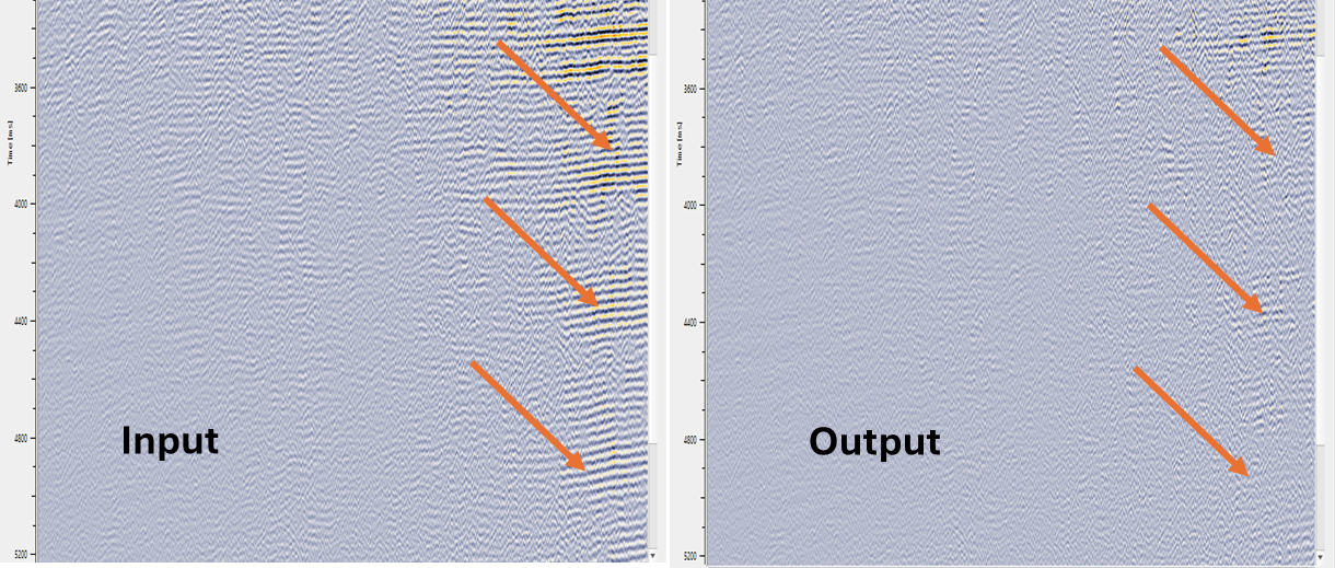
Here is an example workflow, which describes the SRME 2D/3D workflow. In the 1st part, we work on the multiple model prediction. Later in the 2nd part, we read both the input and predicted multiple model and do the adaptive subtraction.

From the above workflow, we've generated the adaptive subtraction(in channel domain) results. In the below image, we can see the input vs output. After the adaptive subtraction, we clearly see that the multiples are attenuated however there is a remnant multiples are there. Try another pass of adaptive subtraction in shot domain to improve the result further.

Selected gather: calculate multiples - Select this option to calculate the multiples for the selected input gather

Selected gather: adaptive subtraction - This options lets the user to perform the adaptive subtraction for the selected input gather from the predicted multiple gather for the selected input gather. This option is only for a visualization of the adaptive subtraction result.

Selected gather: multiples + adaptive subtraction - With a single, it will allow the user to perform both multiple prediction and adaptive subtraction for the selected input gather.

YouTube video lesson, click here to open [VIDEO IN PROCESS...]

Yilmaz. O., 1987, Seismic data processing: Society of Exploration Geophysicist

* * *   If you have any questions, please send an e-mail to: support@geomage.com  * * *