<< Click to Display Table of Contents >> Navigation:  Tutorials > Seismic Processing 2D LAND >                                        SEISMIC DATA QC AND TRACE EDITING

 

 

Usually, seismic data QC includes amplitude and frequency calculation for particular time windows per trace, and seismic processing geophysicist should evaluate the data. Therefore, evaluation consists of creating trace editing set (or library) for quantitative estimation as well as showing QC graphs, maps and schemes to clients. This chapter is spitted into two main parts:

1.Seismic data QC;

2.Trace editing.

 

SEISMIC DATA QC

Seismic data quality control is a special step in processing sequence where geophysicist should analyze new field seismic or legacy data sets. QC seismic attributes calculation is required for a current task. In g-Platform there are following modules for QC attributes calculation and visual estimation:

•QC Attributes;

•QC Attributes calculator;

•Seismic Instantaneous attributes;

•Signal to Noise ratio;

•Spectral Analysis.

 

The main module for QC is QC Attributes, so we are going to use it.

 

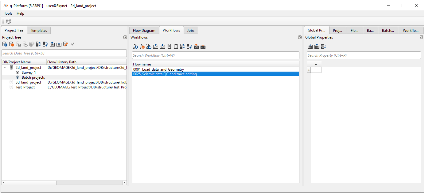
Create a new workflow 0025_Seismic_data_QC_and_trace_edtinig, open it.

 

 

QC Attributes module works with pre-stack and post-stack data sets. It is designed to display color maps of various calculated attributes, alongside a frequency spectrum. The attributes are calculated inside the area defined by the analysis window and inside the noise analysis window. In production seismic processing sequence it is usually when geophysicist should calculate and produce qualitative analysis of the following list of QC attributes: Signal Amplitude, Noise (microseism) Amplitude, Signal to Noise Ratio, Dominant Frequency, Spectrum Width.

 

Add all necessary modules for the first part. Connect input and output data items sequentially:

 

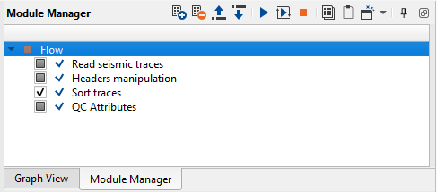
1. Read seismic traces

2. Header manipulation

3. Sort traces

4. QC Attributes

 

 

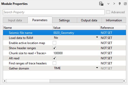
1) Read seismic traces. Load seismic traces from the previous step 0001_Geometry, because this data set has offset values which are required for window definition in QC attributes. Execute the module.

 

Module's parameters:

 

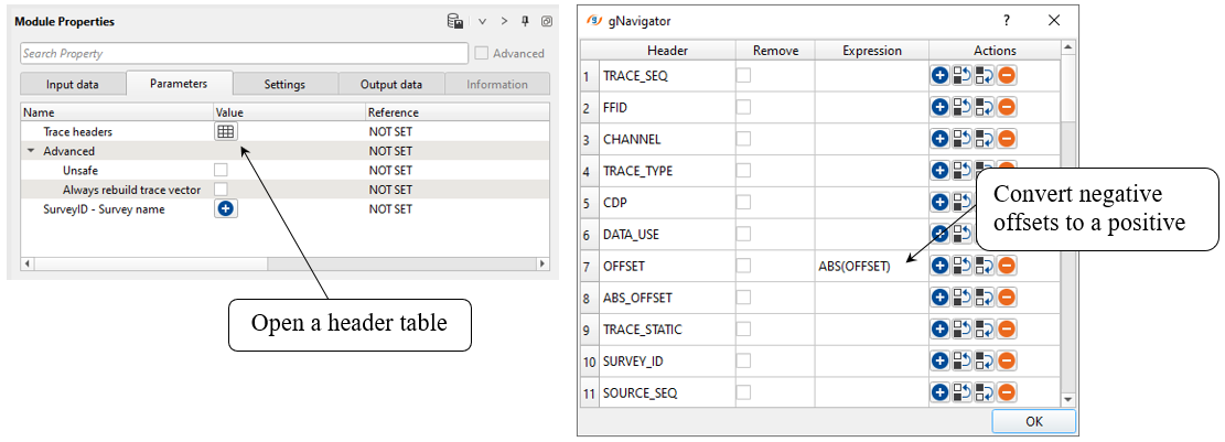
2) Header manipulation. We can modify trace headers. Headers Manipulation module can be useful in doing all sorts of mathematical operations by means of mathematical expressions to change/manipulate the trace headers.

User can use any of the following mathematical operations to create their own equation/expression.

g-Platform uses following mathematical expressions in designing your equation.

•  Mathematical operators (+, -, *, /, %, ^);

•  Functions (min, max, avg, sum, abs, ceil, floor, round, roundn, exp, log, log10, logn, root, sqrt, clamp, inrange);

•  Trigonometry (sin, cos, tan, acos, asin, atan, atan2, cosh, cot, csc, sec, sinh, tanh, d2r, r2d, d2g, g2d, hyp);

•  Equalities, Inequalities (=, ==, <>, !=, <, <=, >, >=);

•  Assignment (:=, +=, -=, *=, /=);

•  Boolean logic (and, nand, nor, not, or, xor, xnor, mand, mor);

•  Control Structures (if-then-else, ternary conditional, switch case);

•  Loop Structures (while loop, for loop, repeat until loop, break, continue).

 

Modify OFFSET header -> covert negative values to positive. We need it for QC Attributes modules:

 

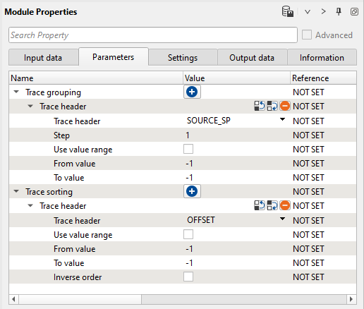
3) Sort traces. QC attributes module requires offset sorted data, so OFFSET is a secondary key in Sort traces module:

 

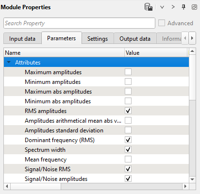
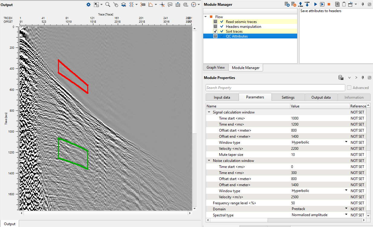
4) QC Attributes. This module calculates many seismic attributes, so it is reasonable to choose only that we really need. Remove unnecessary picks in the check box list:

 

 

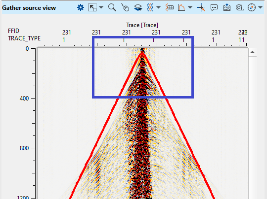
Open vista windows for this module, look at gather and define windows for analysis by setting parameters in the module or use mouse for drawing qc windows:

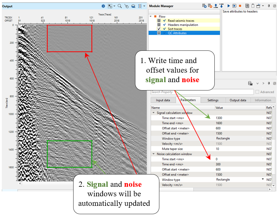
and other parameters:

 

 

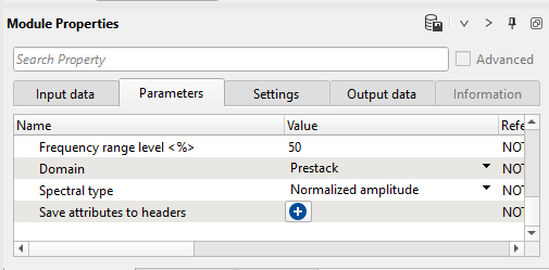
If we need to export QC attributes, use Save attributes to header parameter: add some traces headers -> click on Save attributes to headers function in the modules Action. menu.

 

 

There is an option for hyperbolic window definition: change Window type parameter to a Hyperbolic one, adjust signal and noise window:

 

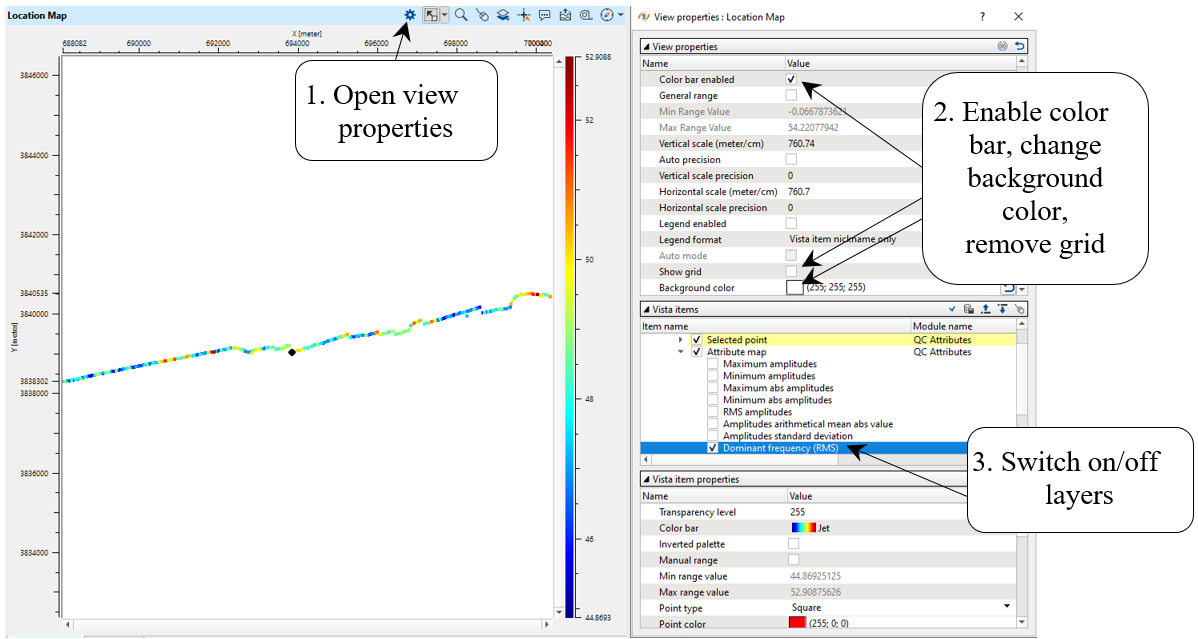
Make sure that you have selected appropriate domain: Prestack or Post stack. Execute the module and check results on the location map. Click on icon of the Location map window. Look at the View Properties window, here we can see all the attributes that were generated by QC attributes module. User should select/unselect the box to display the respective attribute maps.

 

 

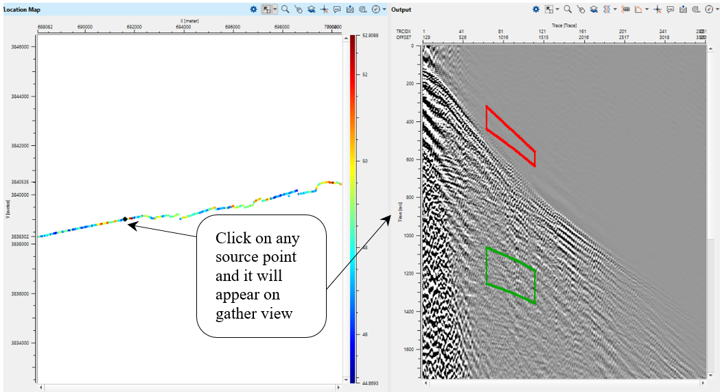
We can choose any point from the location map by left mouse button (LMB) clicking on any source point and gather view will be updated immediately:

 

 

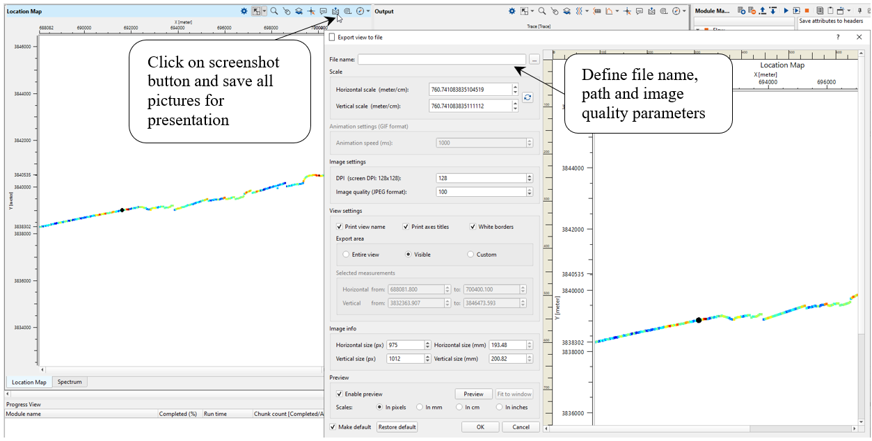
Now we finished with attributes calculation and there is a last point: save pictures for presentation. Use the screenshot function/button :

 

 

 

         TRACE EDITING

 

-------------------------------------------------------------------------------------------------------------------------

  Trace editing is in development. So this chapter is just a short/brief overview of the current

temporary trace editing functionality. A new module will cover auto and manual trace

editing, reverse polarity, empty and auxiliary traces. We recommend you to skip this step

for now, but if are interested in how to do a trace editing in the current version you can go

through it.

-------------------------------------------------------------------------------------------------------------------------

 

Trace editing is also one of the key step in seismic data processing. It should be better to do at the initial stage (preferably). G-Platform provides two modules for this task: Kill empty traces and Geometry application module. In Geometry application module there are three main functions that we need:

 

1. Trace killing/Dead traces

2. Polarity reversal

3. Auxiliary trace marking

 

Trace removing: In order to perform this task, the user should make sure that the geometry is already assigned to the input gather. Once it is confirmed, within the Geometry application, go to the Gather source view window and click on Control item  for options. Select Dead traces source option as shown below and follow the steps as described. 

 

 

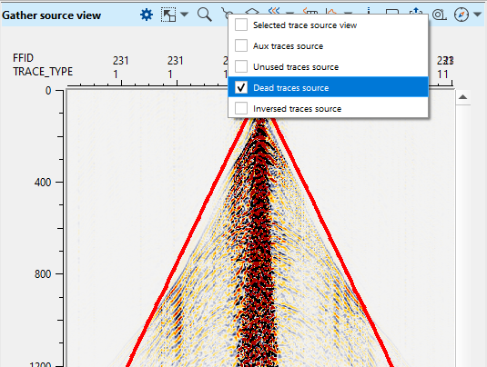
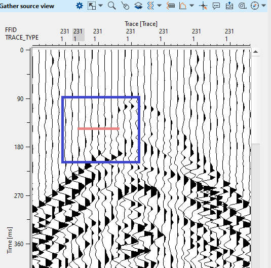
1. Add the trace header TRACE_TYPE. Prior to the trace kill,  TRACE_TYPE of the seismic data is 1 however after marking the trace as dead/kill, TRACE_TYPE changes from 1 to 2 which eventually updates the trace header information. 

 

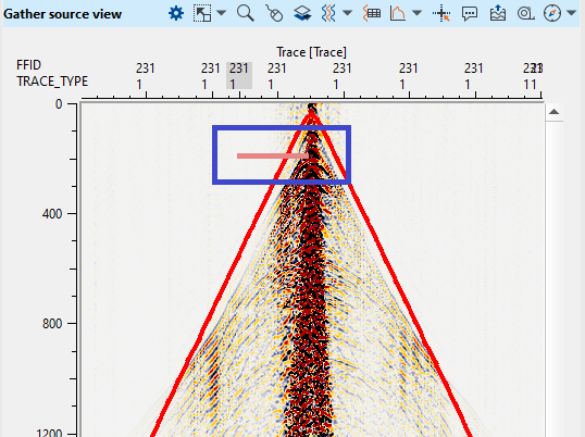
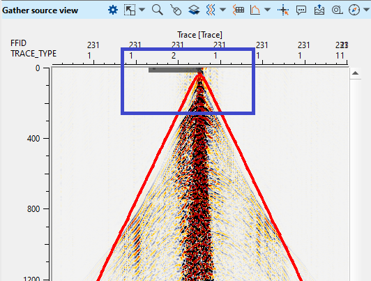
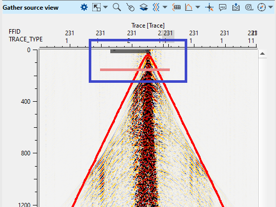
2. To kill/dead any trace in the current shot gather, the user should hold LMB or MB1 and drag the mouse to select N number of traces and release it. It will draw a horizontal line as shown below. Upon releasing the mouse, it will mark these traces as Dead by color code Black (By default) and update the from 1 to 2. 

 

 

     

 

 

 

3. To edit more traces, the user should go to next shot and continue the same procedure to kill/dead the traces. 

4. To reverse the trace kill/dead, the user should hold and drag RMB/MB3 to overwrite the updated trace headers information i.e. TRACE_TYPE from 2 to 1. 

 

   

 

 Please make a note of it that upon marking the traces for killing/dead, DO NOT execute the Geometry application module again. It will overwrite your current changes and put them back to the original trace headers information. It is applicable to all trace editing i.e. trace killing, trace reversal and auxiliary traces. 

 

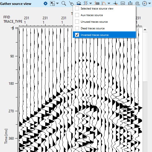
Polarity reversal: To reverse the polarity of any particular trace can be done similarly like the trace kill. Instead of choosing Dead traces source, the user should select Inverted trace source. Prior to the trace reversal, it is advised to change the trace display from Variable Density to Wiggle and Zoom the shot gather to a certain extent to observe the changes.

 

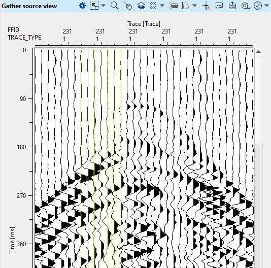
Similar to the trace kill/dead, the user should follow the same procedural steps to mark the traces for trace reversal. Selected traces are marked as YELLOW (by default) in color. 

 

 

   

  

 

 

Next step >>>Spherical divergence.

 

 

 

---

 

If you have any questions, please send an e-mail to: support@geomage.com