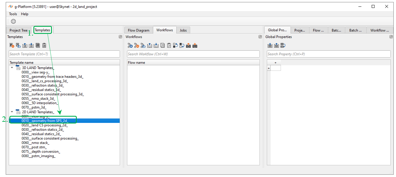
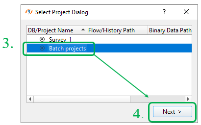
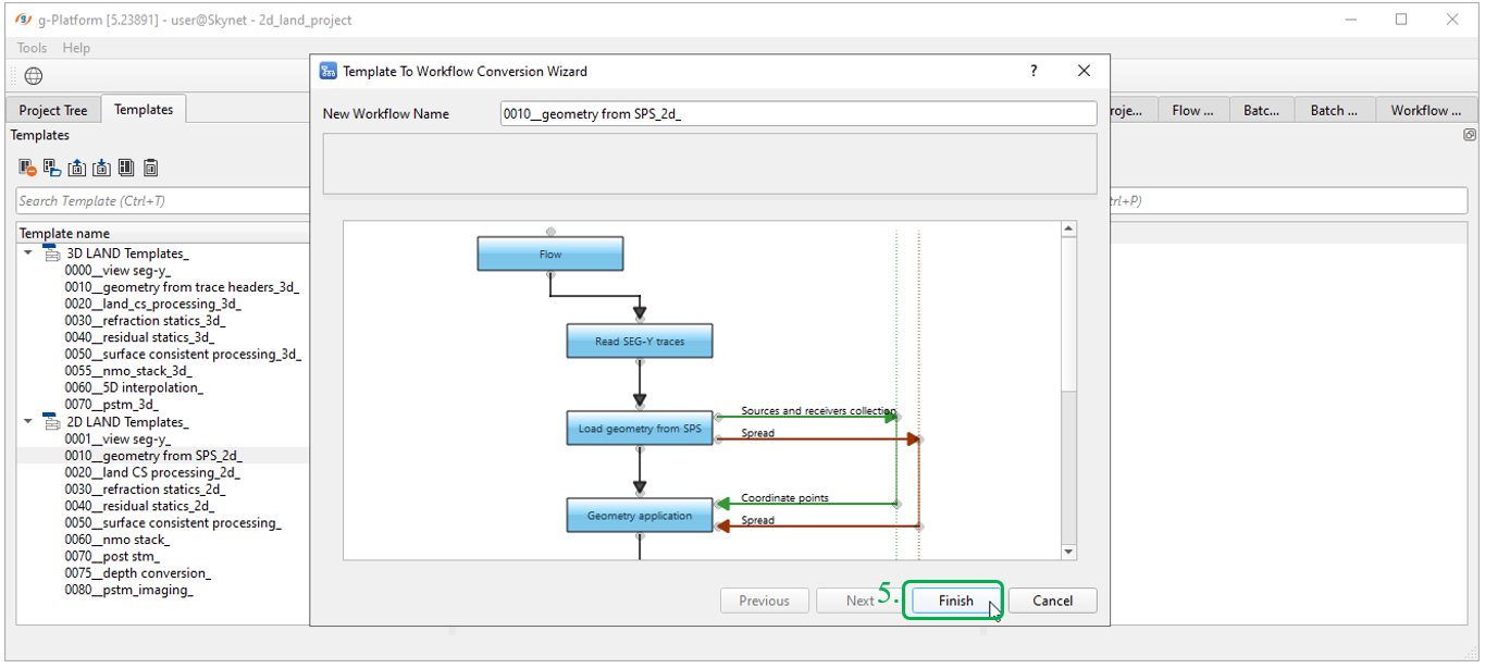
Now we can create the first workflow (or geophysicists usually call it job) for converting input SEGY file into the internal date base and  geometry assignment. There is an option to use jobs examples or templates (see a Templates tab) where you can find all necessary jobs according to the common seismic processing sequences. Therefore, we are going to use it for geometry assignment step. Go to the Templates tab (1) in g-Platform window and double click on 010_geometry_from_SPS_2d_  job (2), in the pop-up window Select Project Dialog -> Batch projects (3) -> Next (4) -> Finish:

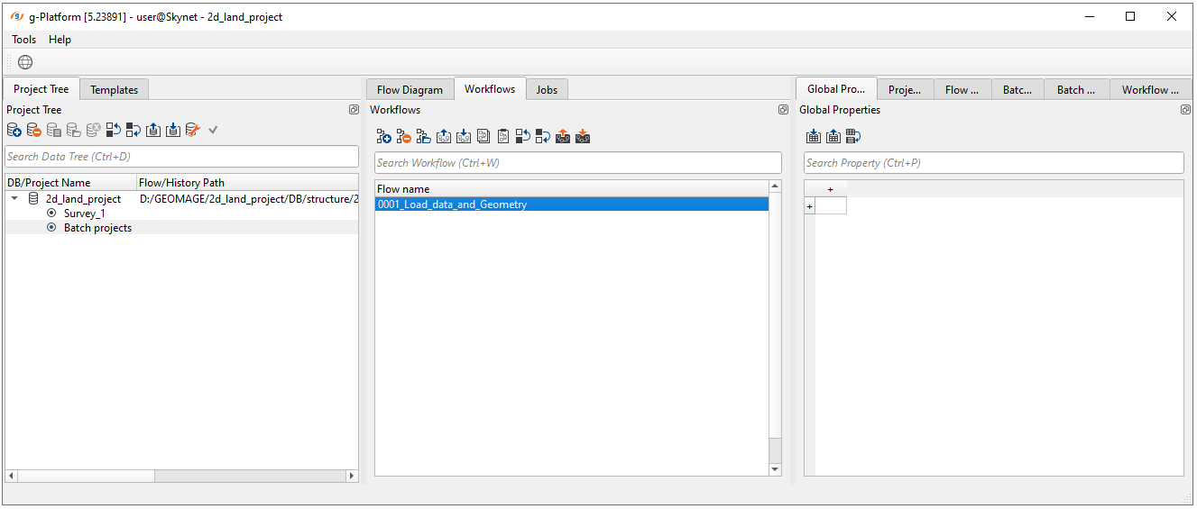
g-Navigator is launched automatically, but you ca just close it for job-renaming. This job now is in your project with the default name which would be better to rename into: 0001_Load_data_and_Geometry. For job renaming: click RMB on the workflow-> Rename (F2):

S-source, R-receiver and X-relation SPS files are included to the training project and you are able to get it from the installation folder: C:/Program Files (x86)/Geomage/gPlatform/demodata/Poland_2D_Vibroseis_LINE_01/:

•Line_001.SPS

•Line_001.RPS

•Line_001.XPS

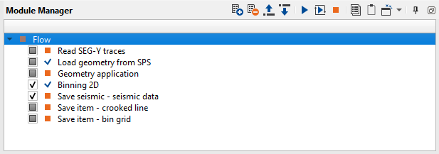
Open the job (g-Navigator window) by double click on it. You will see a typical workflow for reading seismic and geometry assignment:

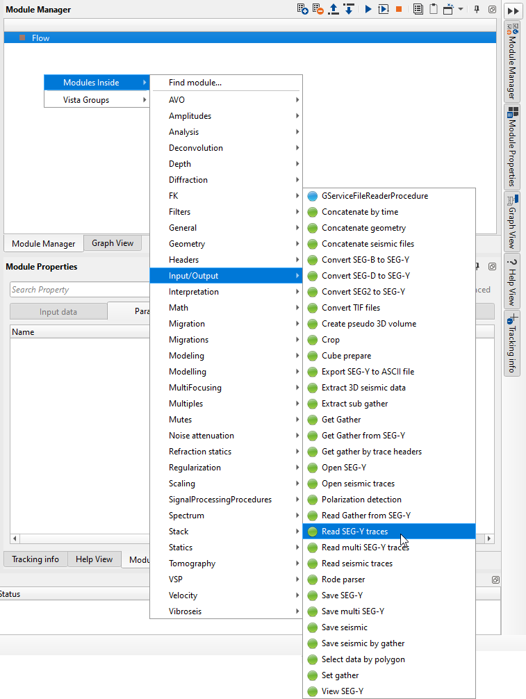
How can we add any module? Let's imagine we have empty workflow, add Read SEG-Y traces module: use right mouse button (RMB) click on the Module Manager area -> Modules Inside -> Input/Output -> Read SEG-Y traces:

Now we know how to any modules to a workflow. Notice that you have many modules for reading input data sets, so use them according to the task. For example, read one SEGY file or several SEGY or SEGD files, etc. In this tutorial we are using seismic data: a vibroseis seismic acquisition Poland 2D line that is accessible on the internet free or it is also included to the g-Platform installation (C:\Program Files (x86)\Geomage\gPlatform\demodata\Poland_2D_Vibroseis_LINE_01).

Let's have look at Read SEG-Y traces modules: input, output data and all visual windows.

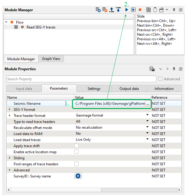
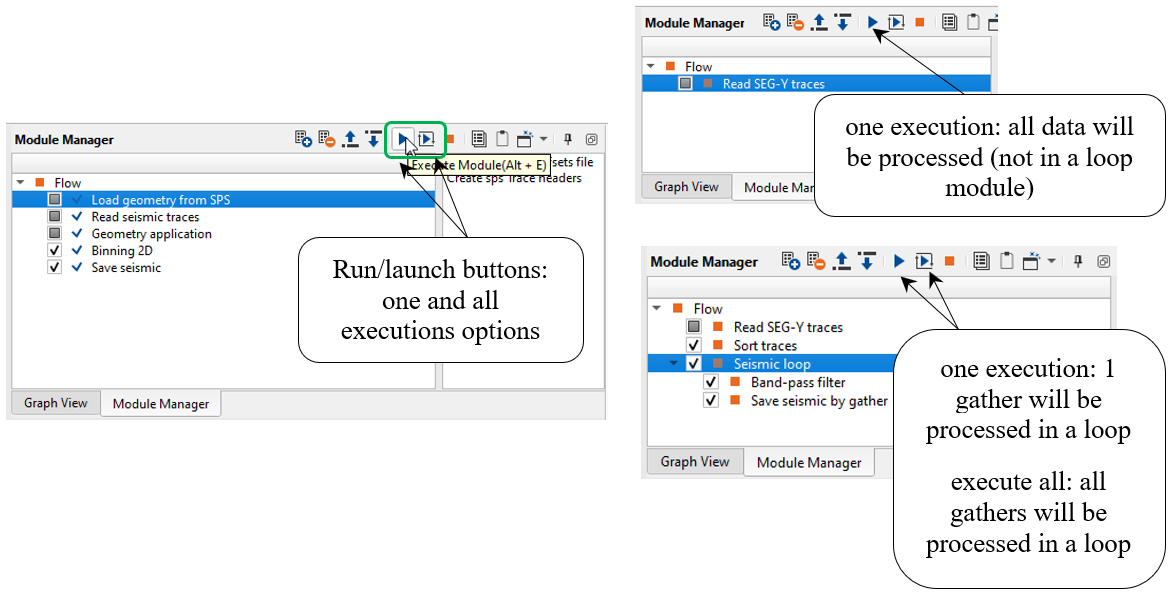
1) Read SEG-Y traces. In the module's parameters we need just select the input file Line_001.sgy via Seismic filename (1) parameter and launch the job by double click on the module or click on button (2). Current 2D line does not require powerful hardware, so performing will be fast. A progress bar and some statistic (errors, log, etc.) during and after calculation you can find at the bottom of GNavigator window.

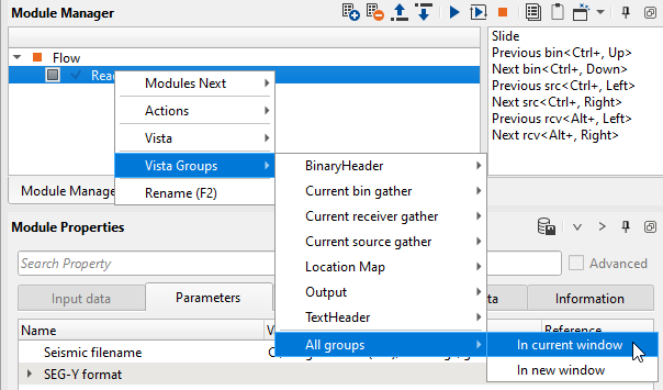
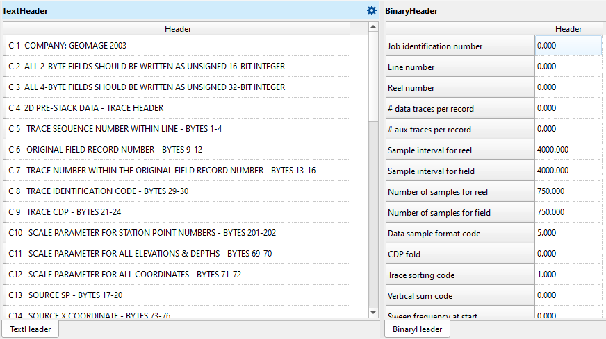
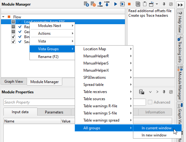
Trace headers were read from the SEGY file and it is possible to check EBCDIC, binary and trace headers. Open all VistaWindows by RMB on the module -> Vista Groups -> All groups -> In current window:

Now only two windows are filled with the information: EDCDIC and binary headers.

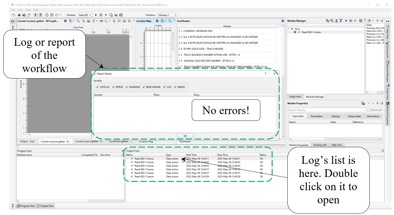
Open a log/report of the workflow:

If we need to visualize more input data (QC windows) from SEGY file it is reasonable to use View SEG-Y module.

------------------------------------------------------------------------------------------------------------------------------------------

WARNING about reading SEGY files!  If the input seismic data is SEGY file:

Do not save seismic from SEGY into internal data base before geometry assignment!!! (i.e. do not use Save

seismic / Save seismic by gather).  

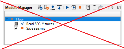
Otherwise, you will lose some trace header information! Therefore ,we must use Read SEG-Y traces, prior

to geometry modules. You should assign geometry before saving traces in DB.

-----------------------------------------------------------------------------------------------------------------------------------------

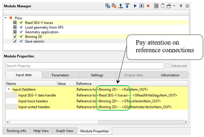
Correct workflow looks like it is shown below (the floe is read SEGY file->geometry assignment-> save seismic into DB - GSD format. Return to our template. Remove other unnecessary modules from the temple job, and use Read SEG-Y traces module that we already prepared previously. Connect all input and output DataItems. The geometry workflow will be consist of the following modules.

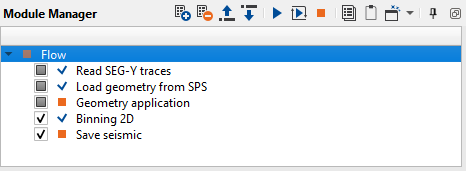
1. Read SEG-Y traces

2. Load geometry from SPS

3. Geometry application

4. Binning 2D

5. Save seismic

-------------------------------------------------------------------------------------------------------------------------------

Data Item is an input or output data set which is located in the Input data and Output data tabs.

Data Item may be seismic traces, sorted headers, velocity model, static corrections and so on.

We can call it Connections.

-------------------------------------------------------------------------------------------------------------------------------

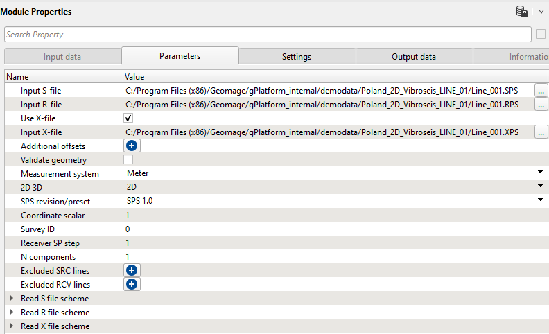
2) Load geometry from SPS module imports SPS files from ASCII into the processing system. There is an option for displaying source and receiver coordinates on the map, S, R, X spreadsheets (tables), inconsistency between SPS files via error tables, source and receiver elevation graph. Execute the module by double click on it or press on this run button  from the upper menu:

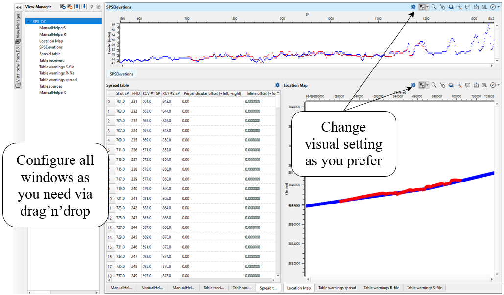
Then add all visual windows called VistaGroups on your work area: press RMB on the module -> Vista Groups -> All groups -> In current window. Now you can look through all visual windows and check SPS files:

Define Input S-file, Input R-file and X-file in the module's parameters:

3) Geometry application is designed for assigning geometry on land and marine 2D/3D seismic data, checking geometry, also manual trace editing is implemented there. The trace headers are filled in accordance with input geometry files, but without binning (binning will be perform on the later stage by using binning 2D/3D modules). The process of geometry assignment is divided into three following steps:

1) Loading and QC geometry files using the Load geometry from SPS;

2) Geometry assignment (Connect geometry from the Load geometry from SPS and the original file trace headers and SEG-Y data handle);

3) QC, correction of applied geometry and optional trace editing.

  -----------------------------------------------------------------------------------------------------------------------------

Geometry Application is a standalone module, and does not need to be run inside a Seismic loop.

-----------------------------------------------------------------------------------------------------------------------------

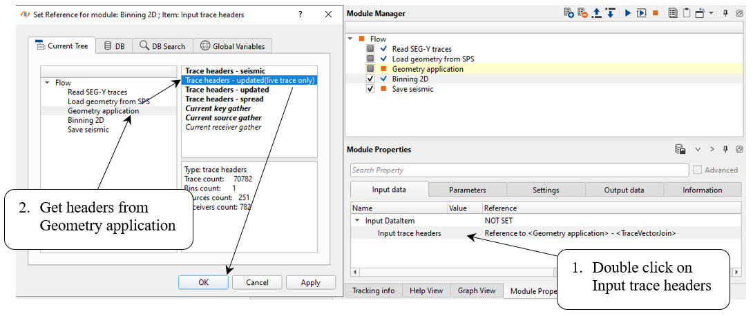
Connect all necessary input DataItems for Geometry application as it is shown below:

Input data:

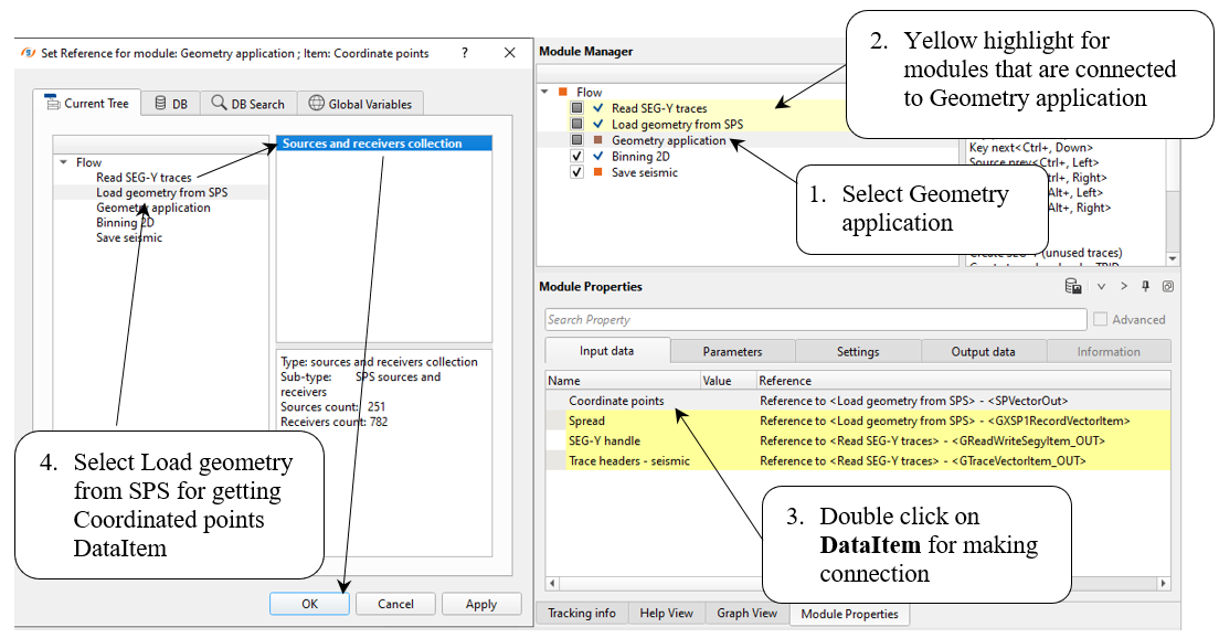
Make all DataIntut connection in the same manner:

•Coordinate points: from Load geometry from SPS;

•Spread: from  Load geometry from SPS;

•SEG-Y handle: from Read SEG-Y traces;

•Trace headers - seismic: from Read SEG-Y traces;

Parameters:

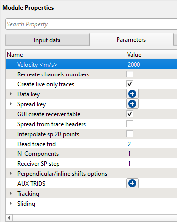
Some  parameters you can change and check the result:

Velocity – set to an approximate Linear Move Out LMO velocity. This is  QC tool and will not be applied to your data;

Dead trid – Change this number if the trace ID marker of your data  for dead traces is something other than 2;

AUX TRIDs – Some data sets have additional auxiliary traces that are marked with special trace IDs. You can indicate that here.

Display all the Vista groups for the module (press RMB on the module-> Vista Groups -> All groups -> In new window.). There are three basic categories of vistas in Geometry application: Tables, Maps, and Traces.

You may click on any entry in a table, or any location on a map, and that point will be highlighted or displayed in all other views. Use the Table Errors Vista to check mis-matches between  geometry files and the seismic data set;

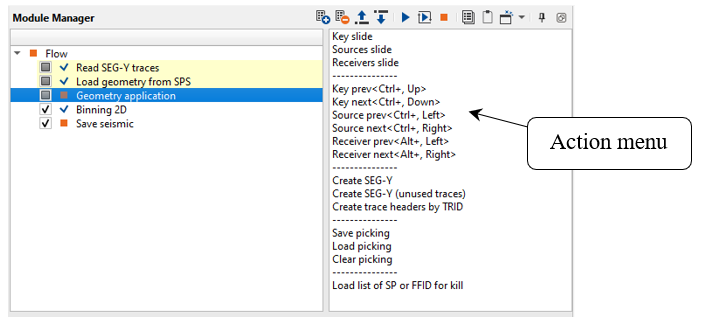
•Use the Action Items associated with Geometry application to view the shots, receivers and field files in auto-mode/movie (Key slide, Sources slide, Receivers slide) or one by one (Key prev, Key next, Source prev, Source next, Receiver prev, Receiver next);

--------------------------------------------------------------------------------------------------------------------------

Not every module has an action menu. Only advanced modules like application or interactive

        have an action menu.  

-------------------------------------------------------------------------------------------------------------------------

•Click on the Map and Table views to view the gathers at particular location:

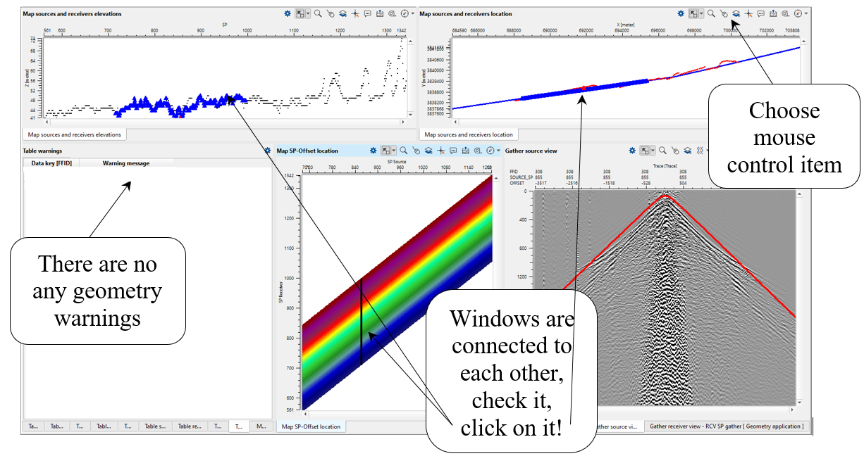
Go through all source gathers and check geometry by comparison first arrivals on traces with the linear velocity function (red line), check the offset distribution on the Map SP-Offset location window, look at all tables and make sure you don't have any critical problem with geometry.

What we have on display:

•Table Errors - vista displays mismatches between the original seismic file and geometry files;

•Table Changed Points - displays points that have been moved, including their new and former positions;

•Table Spread, and Table FFID RAW - display the spread/relation and raw FFID numbers respectively;

•Table Sources, and Table Receivers - display the source and receiver numbers and its coordinates. You may remove shots or receivers (mark all the traces as dead) by right clicking on that entry in the table and selecting Kill Shot or Kill Receiver;

•Table Killed Sources, and Table Killed Receivers - display all the shots and receivers killed (marked as dead) by the user. Killed shots or receivers can be revived by right clicking on an entry in these tables and selecting Revive.

Map views include:      

•Map FFID location, Map Sources and receivers elevations and Map SP-Offset location, which display various cross plots of geometry characteristics;

•Map Sources and Receivers Location display location of shots and receivers on a map, allow to move those points from one location to on another if necessary. See Moving Points. Use these views to verify positions of sources and receivers and move them (see moving points).

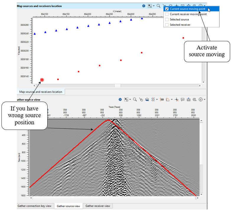
You may move the physical location of a shot or receiver point on the map by using the Map Sources and receivers location.

Use the button on the vista tool bar for the Map Sources and receivers location Vista, choose Current Source Moving Point and Selected Source.

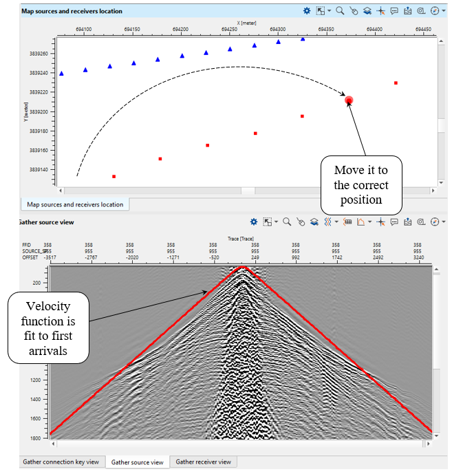
Right mouse click and hold on the source point you would like to move. Drag the point to its new location. The previous location of the source will be indicated by its original marker (default: Red triangle), and the new location will be indicated with new marker (by default, a semi-transparent red circle).

When you move some source point, the Velocity display on the Gather Source view will be updated and it reflects a new source point location.

The source point marker will be updated with its new location when you click on the new point again, or on a different source point.

The new position will also be reflected in the Table Changed Sources.

Try to move the point so that the velocity display aligns with the traces on the Gather view. The peak of the velocity function should match up with the nearest first arrivals – this is a good indication that your source point is positioned correctly.

Gather connection key views:

•Gather key, Gather Receiver, and Gather Source, which display the traces of the currently selected key, receiver, and source. You may edit individual traces in these views.

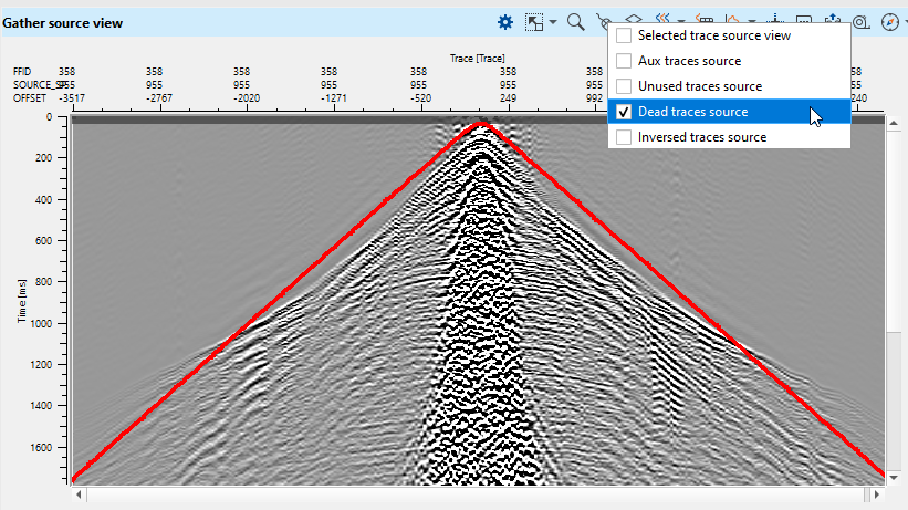
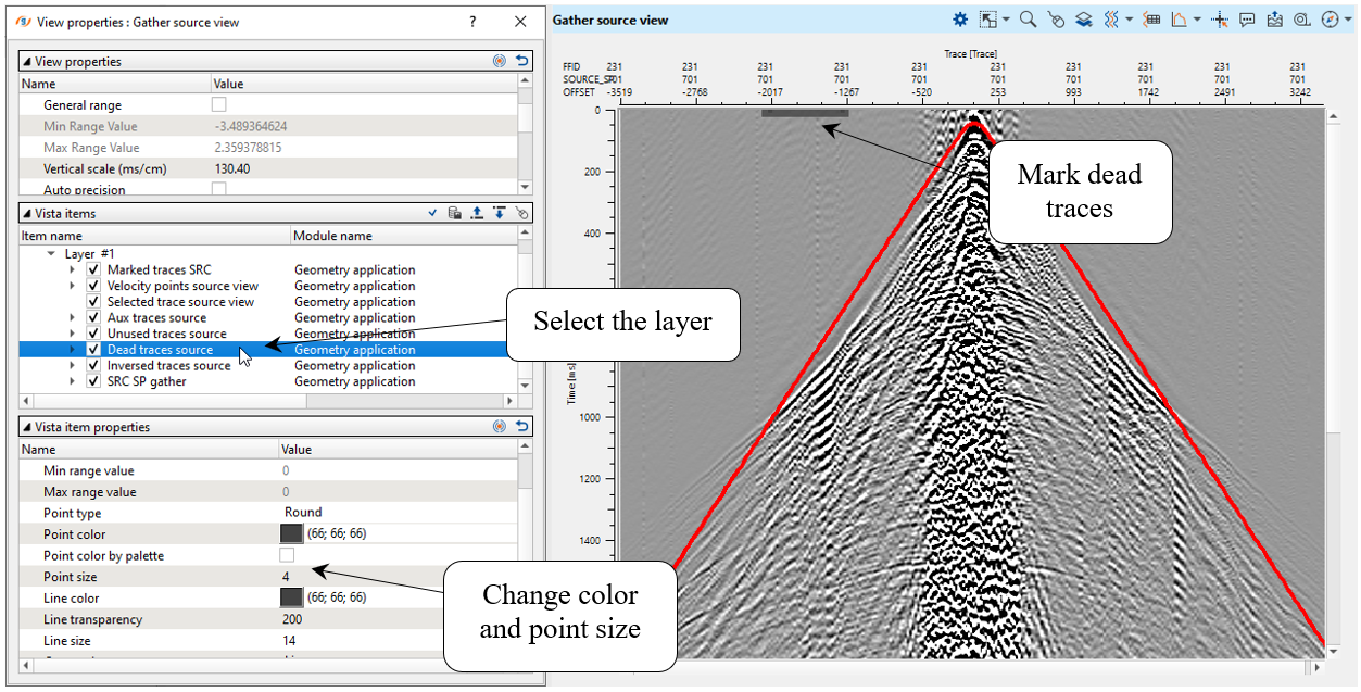
•Use the Trace Editing feature to reverse trace polarities, or mark problem traces as dead.

For trace editing: choose gather display source, receiver or sorted gather, select the type of trace marker you would like to set. Make sure only one option is checked off at a time.

1. To set traces as dead, and remove them from the dataset, choose Dead Traces;

2. To reverse the polarity of traces, choose Inversed;

3. To set the unused marker, choose Unused;

4. To set the auxiliary flag, choose Auxiliary.

To set a marker, right click with the mouse, or right click and drag across several traces.

To apply those markers to your data, run the geometry application module.

Traces will not be removed or changed until you save the resulting data set using Save Seismic or Save SEG-Y.

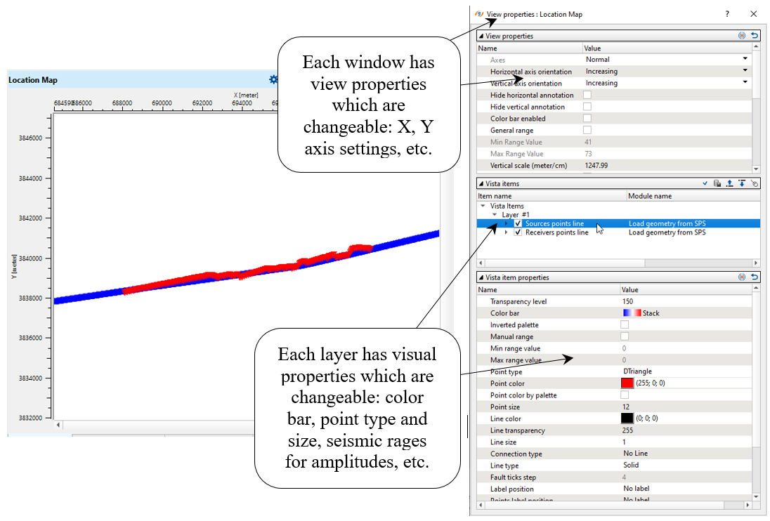
Go into the Vista properties of the view to adjust the size and color of the trace markers, to make it easier to see which traces are flagged:

Once you have performed all geometry edits, run the Geometry Application module. Geometry will be assigned: output traces headers are updated, dead traces are removed from the data set.

4) Binning 2D. Now we have geometry information from SPS files inside seismic trace headers, so the last step is to calculate slalom line for binning 2D and update CMP numbers and coordinates.

This module creates geometry for 2D seismic data set where traces are grouped together by their sub-surface positions into common midpoints (CMP). For visual quality control, the module creates several vista views for binning quality control.

The binning process consists of the following steps:

1. Filter  midpoints by maximum trace offset value. Only midpoints that have an offset less than or equal to a user specified value will be used.

2. Build the grid. A direct line is drawn from the first source/receiver location to the last source/receiver location. The line is then divided into segments, with each segment being the grid size of the slalom line as defined by the user.

3. Build the slalom line. The set of midpoints are divided into groups using the grid increment previously defined. The center point of each midpoint group is determined, these points are connected and become the slalom line.

4. Smooth the slalom line by using the slalom smooth parameter and the topography smooth window parameter.

5. Build a crooked line using the crooked line increment parameter. The first point of the crooked line is the first source/receiver bin center point and the last point of the crooked line is the last source/receiver center point location.

6. Build a stack line using the stack line step parameter. This is the CMP spacing. The first point of the stack line is the first center point and the last stack point is the last center point. The user assigns the number of the first CMP and these will then increment by one

7. Filter midpoints with a maximum distance between the MP and CMP point parameter.

Set up all necessary module's parameters and launch the job, check results:

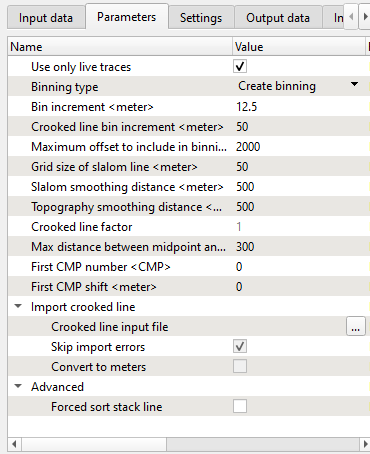
Parameter definition:

There are several options to define binning (Binning type):

• Create binning – create a sub-surface geometry using parametrization of current module;

• Import binning from SEG-Y – use a sub-surface geometry from specified SEG-Y input data set;

• Import existing crocked line from ASCII file - it allows to import an existing crooked line from an ASCII file. For example, a crooked line which was built and used by other processing companies/software’s during data processing. The advantage of this option is in using all information of binning from the input file, the parameters of the module in this case are not in use;

The crooked line file in ASCII format should include the following information, 3 columns: CDP number, CDP-X and CDP-Y coordinate of previous result.

Bin increment

Distance between (CMP) points of stack line;

Crooked line bin increment

Distance between points of a crooked line;

Maximum offset to include in binning

Only midpoints that have an absolute offset distance less or equal to the specified value will be used in the binning process;

Grid size of slalom line

Grid size that is used for slalom line building;

Slalom smoothing distance

Smoothing distance over which to smooth the slalom line;

Topography smoothing distance

Smoothing distance over which to smooth the topography line;

Crooked line factor

If import binning from txt file option is chosen, this parameter is used as decimation factor;

Max distance between midpoint and CMP point

Only midpoints whose distance to the bin center point will be included the bin;

First CMP number

It is recommended that this parameter be 2 times the number of the first live receiver station number. That makes it easier to relate a CMP number to its position relative to the station numbering of the line;

First CMP shift

Shift the first CMP point, meters;

Import crooked line:

Crooked line input file - Full path name of the text or SEG-Y file that will be used for binning if a Binning type option other than Create binningis used;

Skip import errors - If checked, ignore errors of importing crooked line;

Forced sort stack line - If checked, reverse the stack direction.

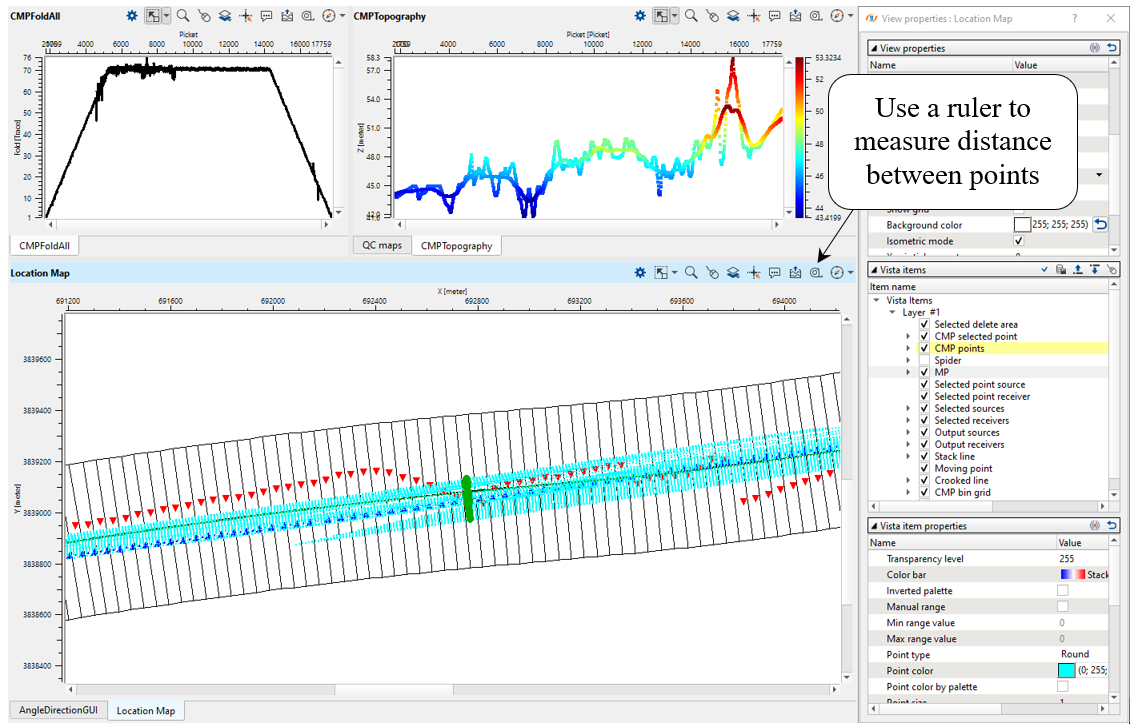
Add all vista group in a new window. Look at CMPTompography window, there are two elevation lines: original relief and smoothed one. Smoothed elevation it is a float datum that you will use on the further processing steps, for example velocity estimation, etc. More detailed review of datum planes will be in the chapter Datum planes.

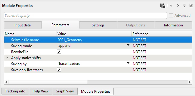
5) Save seismic. The final step in this workflow is saving seismic traces with all geometry information in headers: SOURCE_X, SOURCE_Y, RECEIVER_X, RECEIVER_Y, OFFSET, SOURCE_SP, RECIVER_SP, SOURCE_ELEV, RECEIVER_ELEV, CDP, BIN_X, BIN_Y, BIN_ELEV, ...

Write a name for the output data set 0020_Geometry and execute the job.

Input data:

Parameters:

      -----------------------------------------------------------------------------------------------------------------------------------------------------------------

  Be careful with the Saving mode = Append, in this case each time you execute module, each time it is adding seismic traces to the previous file, in other word 2 times run will lead to duplicates traces in output 0001_Iput_SEGY_2D file. To avoid the problem use RewriteFile mode.

-----------------------------------------------------------------------------------------------------------------------------------------------------------------

We can stop at this point and go the next chapter or continue with extra QC module which is might be useful to check geometry.

Next step >>> Seismic data QC and trace editing

      If you have any questions, please send an e-mail to: support@geomage.com    

   Load Geometry from SPS - Geomage g-Platform - YouTube

        Geometry Application - Geomage g-Platform - YouTube