 | LOAD DATA AND GEOMETRY ASSIGNMENT |
|
<< Click to Display Table of Contents >> Navigation: Tutorials > Seismic Processing 3D LAND >
|
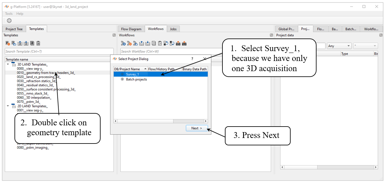
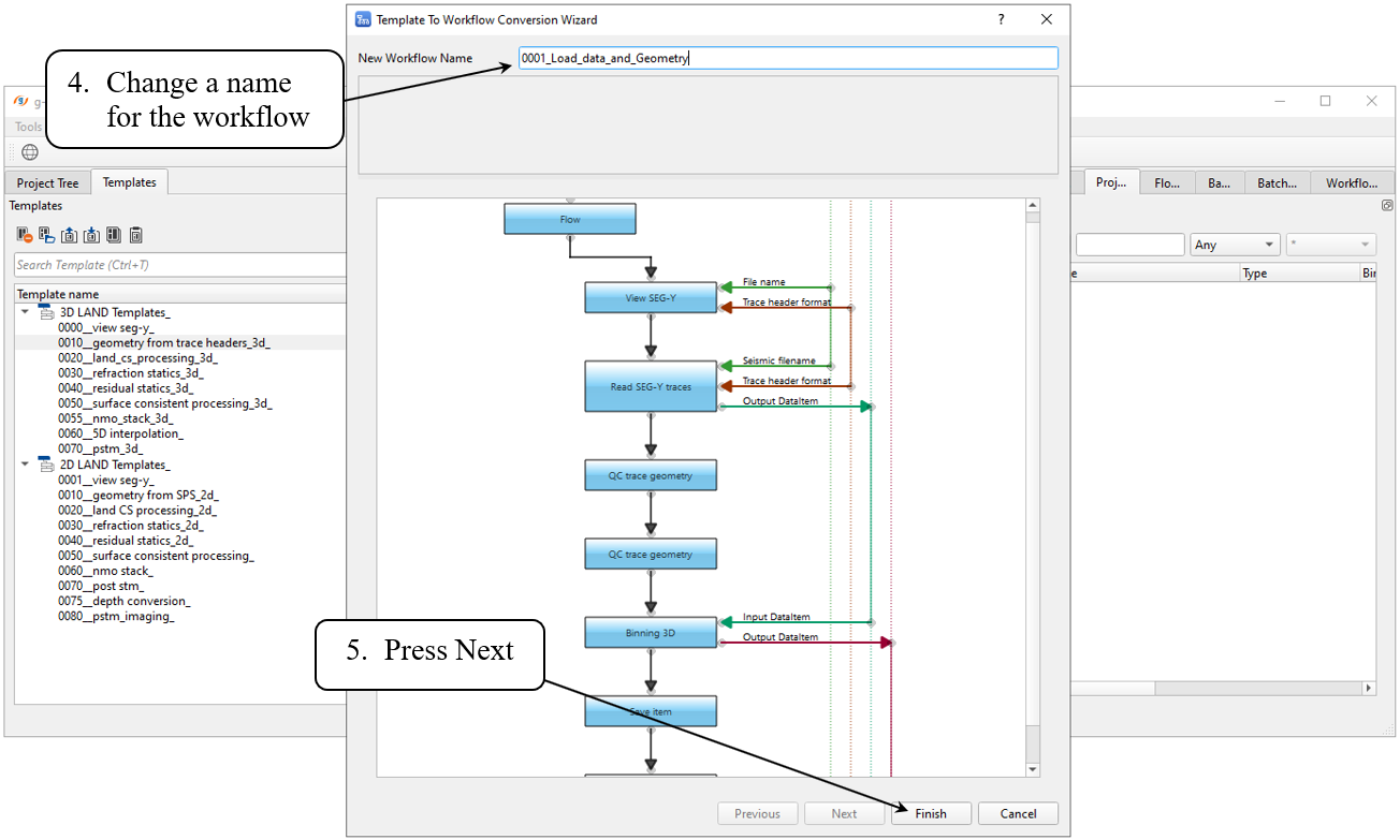
Now we can create the first workflow (or geophysicists usually call it job) for converting input SEGY file into the internal date base and geometry assignment. There is an option to use jobs examples or templates (see a Templates tab) where you can find all necessary jobs according to the common seismic processing sequences. Therefore, we are going to use it for geometry assignment step. Go to the Templates tab (1) in g-Platform window and double click on 010_geometry_from_trace_headers_3d_ job (2), in the pop-up window Select Project Dialog -> Batch projects (3) -> Next (4) -> Finish:
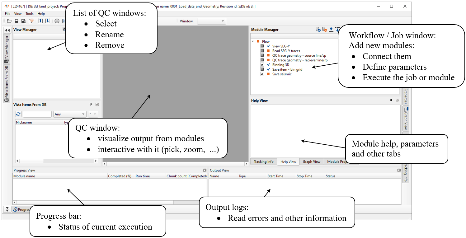
g-Navigator application is automatically opened, let's have a look what we have here: most of the tabs and windows we can move, change their location as we prefer:
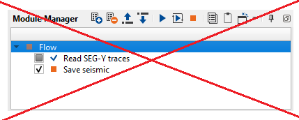
Go to the workflow and remove View SEG-Y and QC trace geometry modules, because it is only for SEGY file and its traces headers QC and we can skip it:
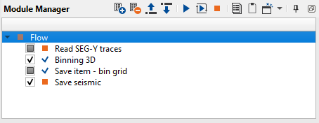
There are a few modules, we will set parameters for each one consequently:
1.Read SEG-Y traces
2.Binning 3D
3.Save item - bin grid
4.Save seismic
1) Read SEG-Y traces is designed to read seismic traces from SEGY files, and make them available for use inside g-Platform. By default, Read SEGY traces will not display the input traces of your SEGY, even when the module has run successfully. To view traces, use View SEGY instead.
Notice that you have many modules for reading input data sets, so use them according to the task. For example, read one SEGY file or several SEGY or SEGD files, etc. In this tutorial we are using seismic data: Teapot Dome 3D that is accessible on the internet free (http://s3.amazonaws.com/teapot/npr3_field.sgy. We should download this file and save it on local work station. Teapot dome 3D data contains both pre and post migrated data. We are using pre-stack data (3D raw shot gathers, size = 5.7 Gb).
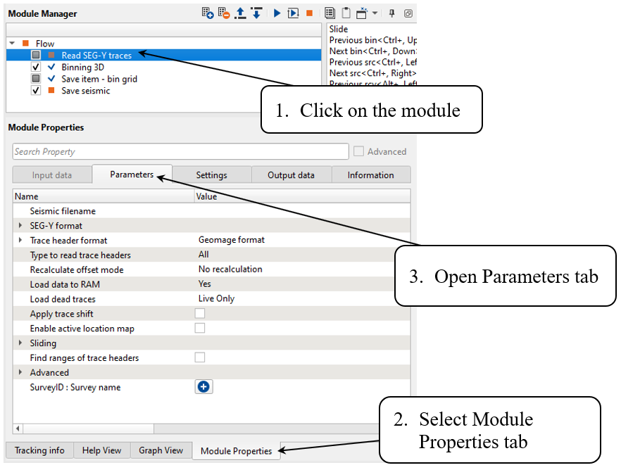
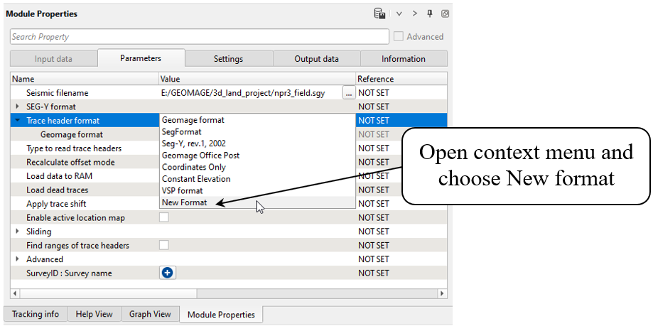
In this 3D volume, geometry is already assigned. To get the already existing trace headers information, we should create a new trace header format by clicking on the Trace header format -> New Format.
Select the first module and go to the parameters tab:
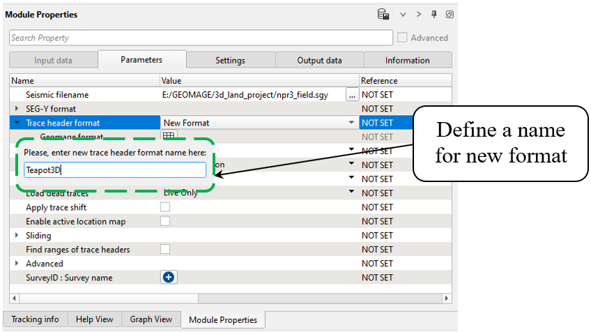
Open npr3_field.sgy seismic file and define a name for the new trace header format and press enter:
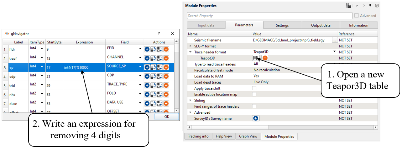
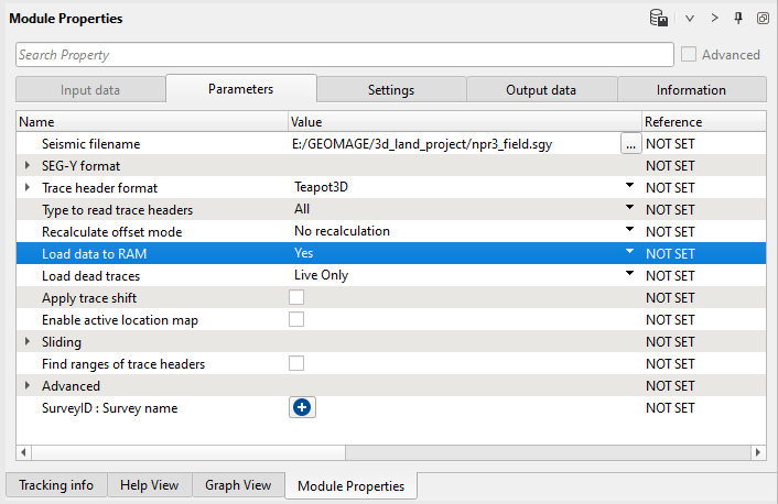
In the module's parameters we need just select the input file npr3_field.sgy via Seismic file name (1)
Parameters:
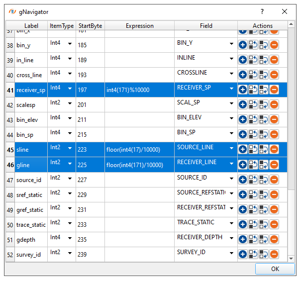
Header table provides an option for changing bytes of any trace header, as well as applying mathematical expressions. We need to modify SOURCE_SP, RECEIVER_SP, SOURCE_LINE and RECEIVER_LINE. Source number is complex value which is consists of source point number and source line, so we need to split them out and write into different trace headers.
Modify other trace headers in the same manner:
Load seismic data to RAM. If this option is selected, the program will load all of the traces to RAM memory. Traces can also be displayed by the module. However, only do this if the data set is small enough to fit in the RAM memory of your system. This option is used in current workflow mainly for saving traces in the end of the flow, because it is required to read seismic traces. There 2 options for reading data set: 1) use Seismic loop module for gather processing (read and write each gather consequentially); 2) load all seismic data set into RAM.
Finally, we have these following parameters:
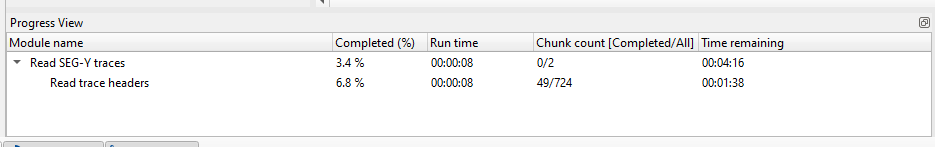
Execute the module by double click on the module or click on button ![]() . Even though it is a 3D volume, it does not require powerful hardware, so reading the data doesn't take much time with a modern work station or laptop. A progress bar and some statistics (errors, log, etc.) during and after calculation you can find at the bottom of g-Navigator window.
. Even though it is a 3D volume, it does not require powerful hardware, so reading the data doesn't take much time with a modern work station or laptop. A progress bar and some statistics (errors, log, etc.) during and after calculation you can find at the bottom of g-Navigator window.
Check the progress bar at the bottom of g-Navigator window:
Open log/listing:
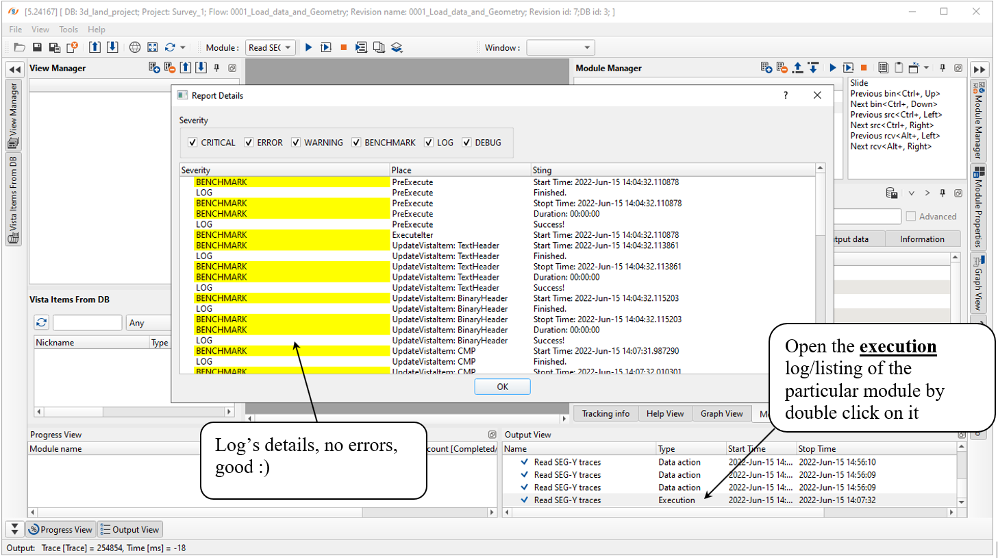
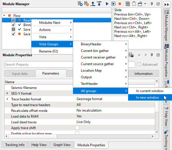
Trace headers were read from the SEGY file and it is possible to check EBCDIC, binary and trace headers. Open all VistaWindows by RMB on the module -> Vista Groups -> All groups -> In current window:
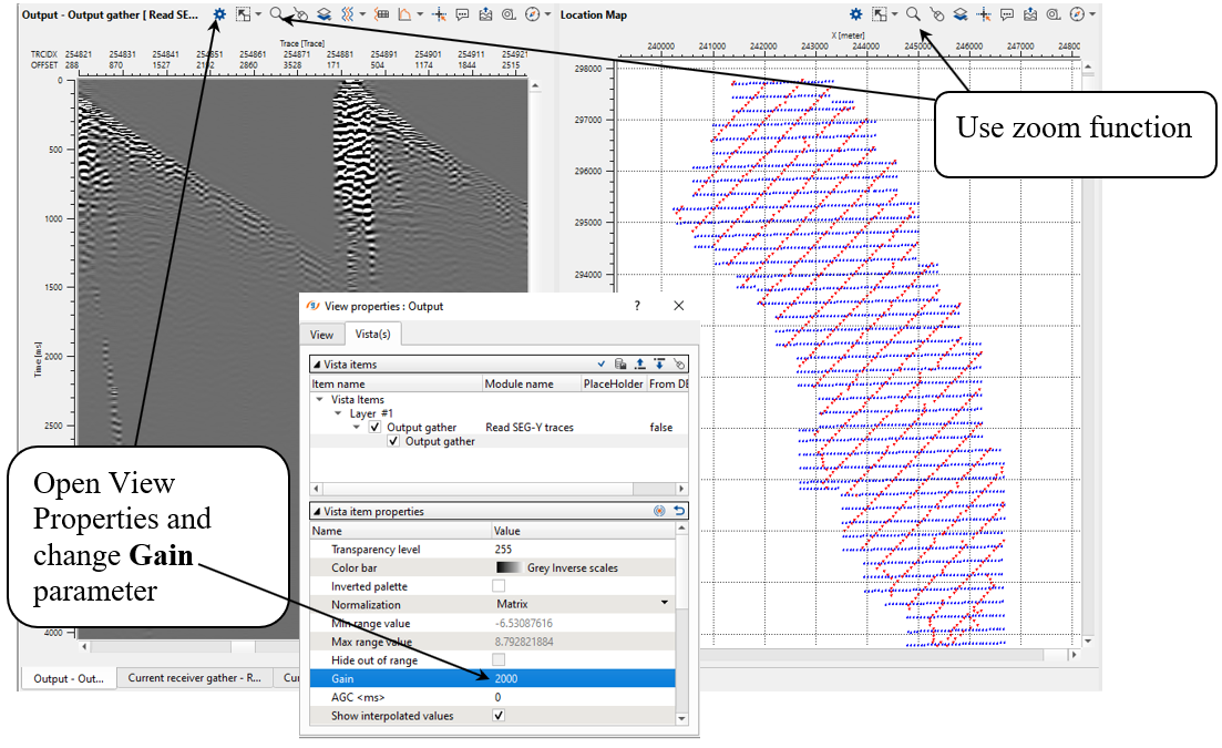
As we mentioned earlier that, this particular input data is having all the geometry information, we can see the location map, seismic data, the EBCDIC and Binary headers information as well.
Output gather and Location Map windows:
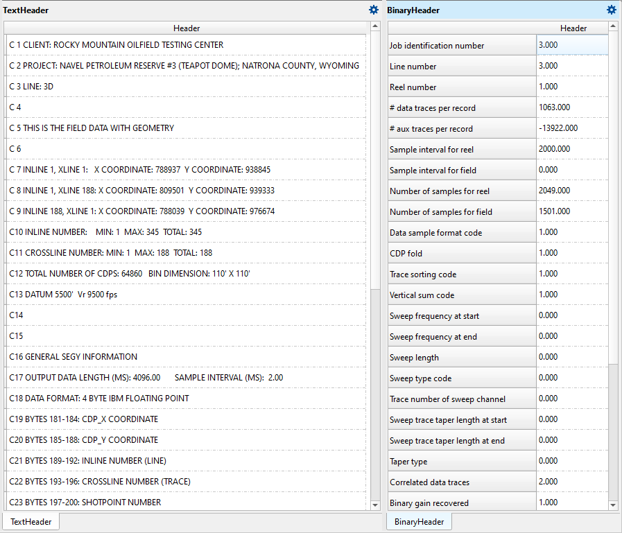
TextHeader and BinaryHeader windows:
![]() If we need to visualize more input data (QC windows) from SEGY file it is reasonable to use View SEG-Y module
If we need to visualize more input data (QC windows) from SEGY file it is reasonable to use View SEG-Y module
---------------------------------------------------------------------------------------------------------------------------------------------------
![]() WARNING about reading SEGY files! If the input seismic data is SEGY file:
WARNING about reading SEGY files! If the input seismic data is SEGY file:
Do not save seismic from SEGY into internal data base directly, i.e. before geometry assignment!!!
(i.e. do not use Save seismic / Save seismic by gather).
Otherwise, you will lose some trace header information! Therefore ,we must use Read SEG-Y traces,
prior to geometry modules. You should assign geometry before saving traces in DB.
-----------------------------------------------------------------------------------------------------------------------------------------------------
2) Binning 3D. Binning for 3D seismic data and QC mapping. This module performs binning for 3D seismic data, the input data are seismic traces with geometry updated to the trace headers. (Source and receiver X,Y,Z coordinates and station numbers). Binning 3D creates a smoothed topography surface (CMP) using user specified parameters and saves it to the trace headers for use with MultiFocusing and velocity analysis. It also produces an non-smoothed version of the topography as well. The module produces several other QC’s to check the positioning of the grid bin centers relative to the midpoints in a bin. Other QC’s generated and available as Vista views are a fold of coverage map, minimum and maximum offset distance in a bin, bin center to bin centroid distance, bin center to bin centroid distance of X and Y coordinates, a rose diagram giving some azimuthal information, statistical information about the grid (the number of inlines, crosslines, size of area, etc.), a source/receiver midpoint/bin center location map as well as the bin topography map (smoothed and non-smoothed).
Connect all necessary input data items:
Input data:
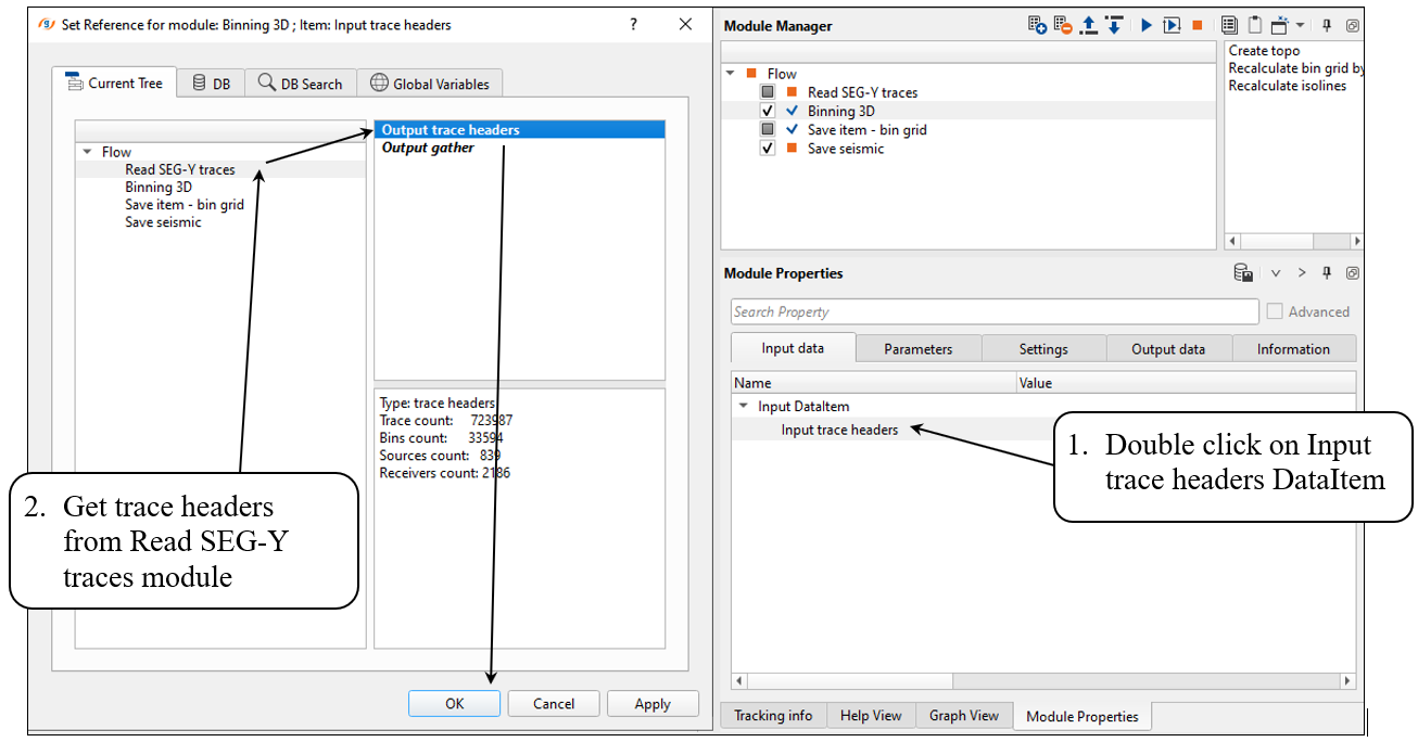
The input seismic data set does have SPS-geometry information in trace headers, so we just need to perform a binning procedure which is required in g-Platform system. Even though input traces already have bin information, we have to apply binning, because those virtual geometry is used internally in the project. Therefore, Binning 3D module uses original geometry information from the trace headers. Otherwise, we have to read SPS files ad use Geometry application prior binning process. Unlike Binning 2D, Binning 3D requires additional information. It requires the Bin starting point. It also requires the 3 corner points along the inline and cross line directions. Recalculate bin grid by input data can automatically calculates the bin starting point and other corner points from the input trace headers information.
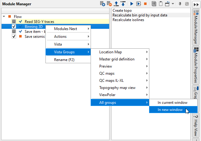
Open all visual vista window groups in the new window from the Binning 3D module, by using a context menu (click RMB on the module and select a particular option):
Now they are empty, because we haven't apply any of function (actions menu or module execution):
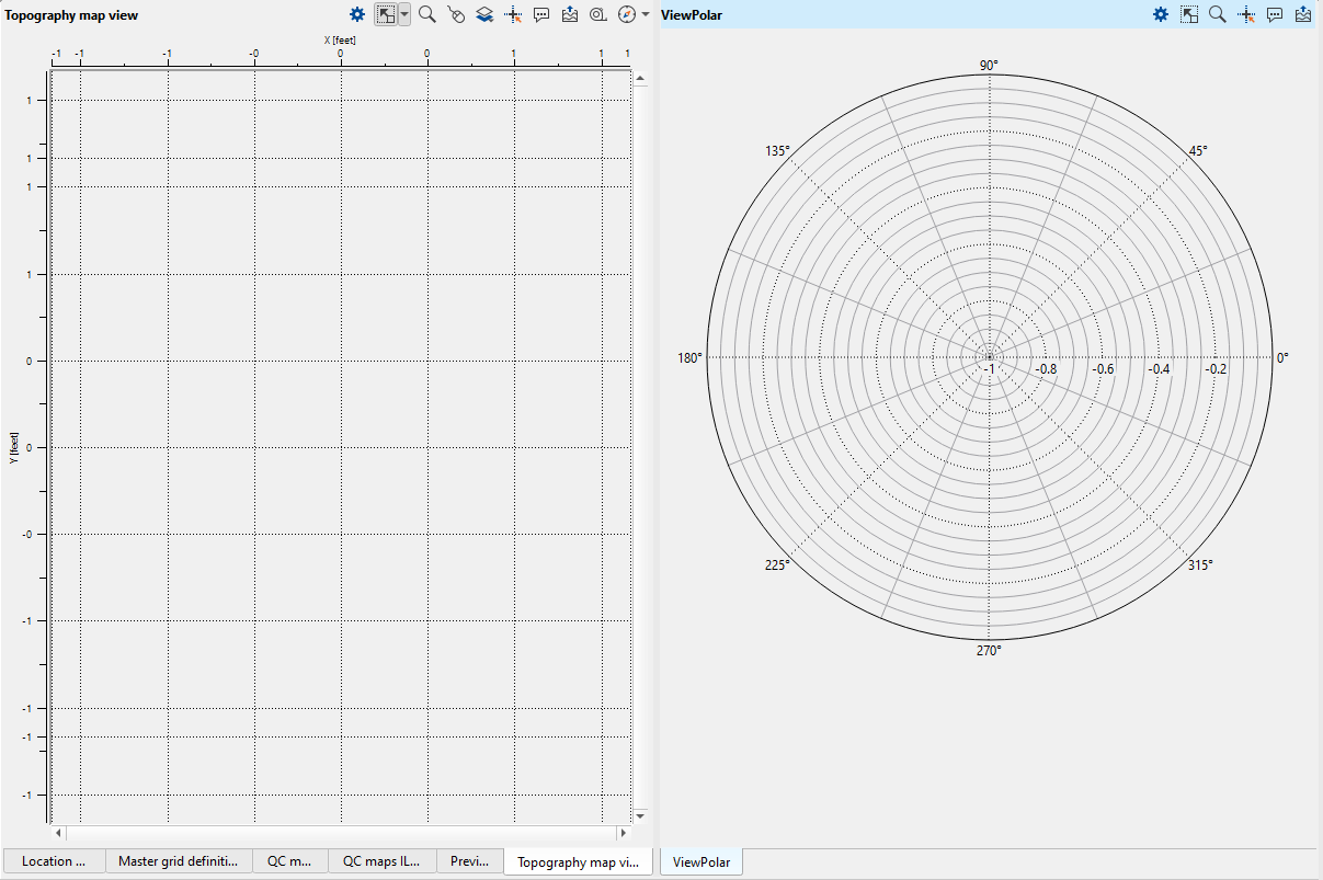
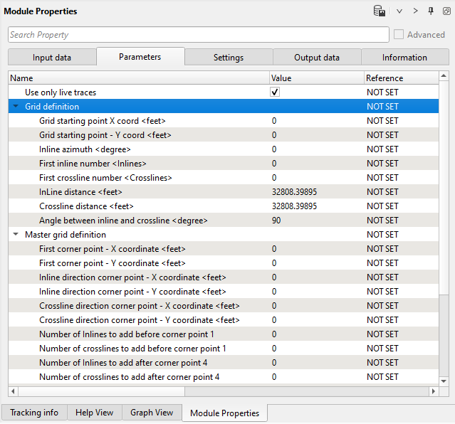
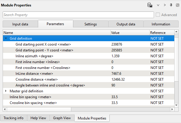
Look at the grid parameters, now they are undefined:
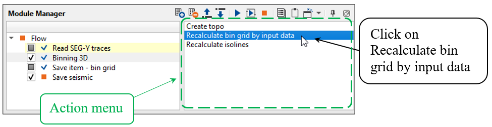
Use the Recalculate bin grid by input data action item by clicking on it in the action menu. Action menu is an menu with extra functions implemented in some complex modules:
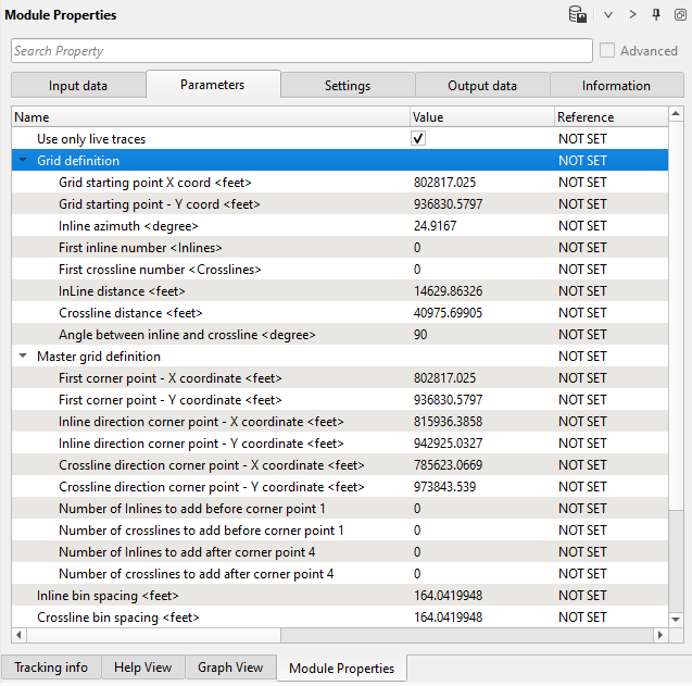
And check the grid parameters again, now they are automatically were calculated:
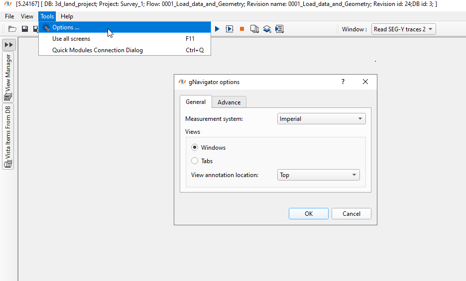
Teapot dome 3D data set is acquired in Imperial system. To change the measurement systems from the metric (By default) to the imperial system we should change it as described below:
If you would like to change it to Imperial: go to the g-Navigator window and choose Tools -> Options. Select the Measurement system from the drop down menu and click OK:
Return to our workflow. Go to the vista windows, the grid appeared:
Open the Location map tab:
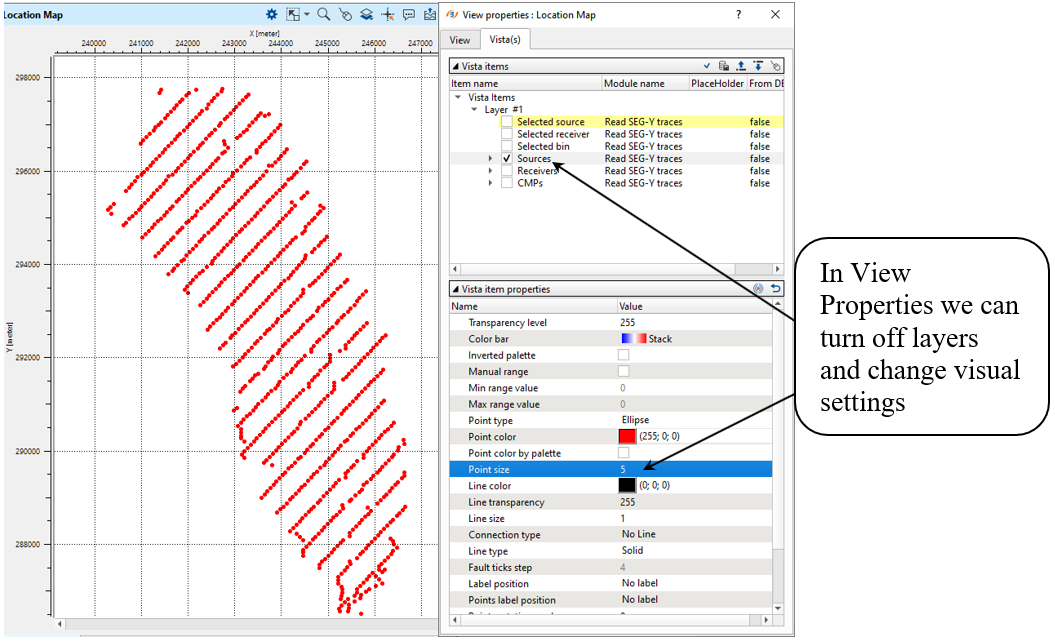
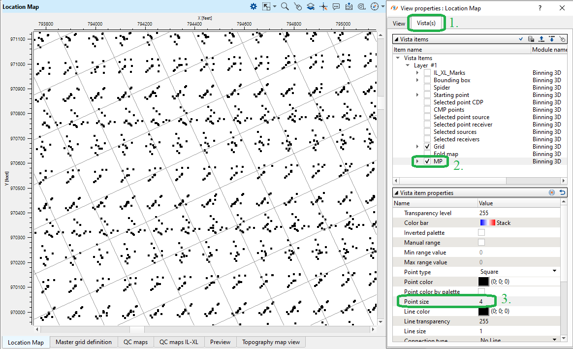
Zoom some area in the center of the survey and switch off unnecessary visual grid (do not be confused: not a geometry grid) by using a View properties:
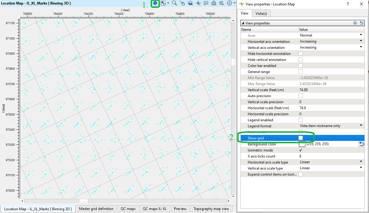
Configure visual setting for layers: grid lines, CMP points, Sources, etc.
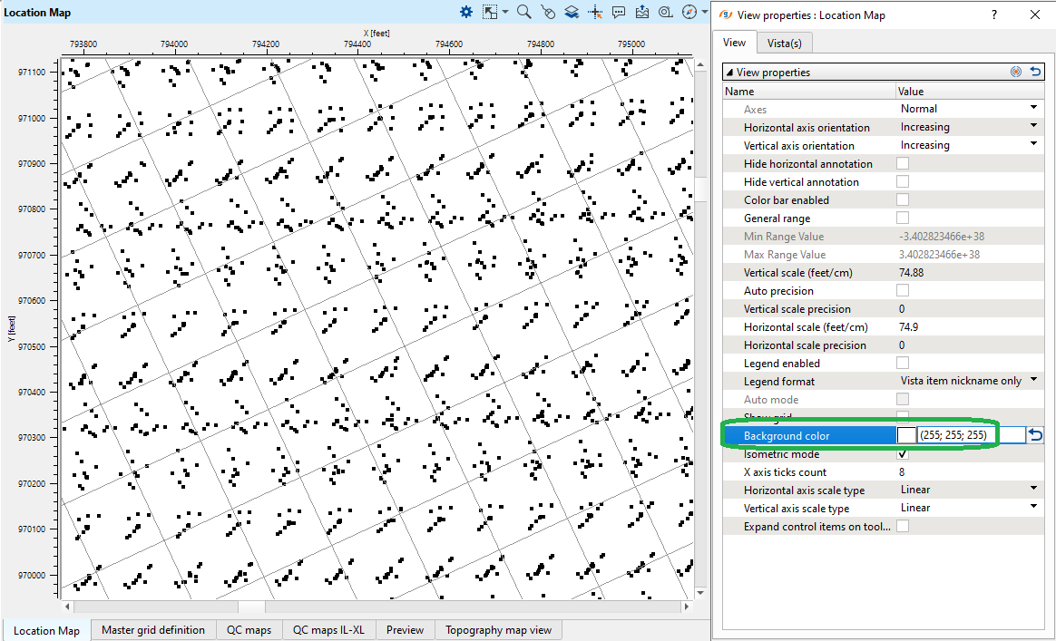
Background color does have a small issue: need to select another color and then select white color again:
You can turn off any layers and change its visual effects by using another tab called Vista(s):
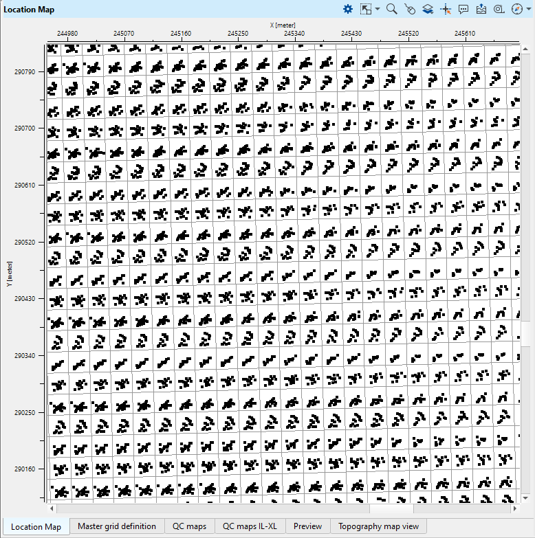
Obviously, the resulting binning is not acceptable due to the fact that we have unconventional acquisition (source lines are not perpendicular to receiver lines). Therefore we have modify the grid. Change gird' azimuth, starting point and bounds as shown below:
Now all common middle points are in the center of a bin position:
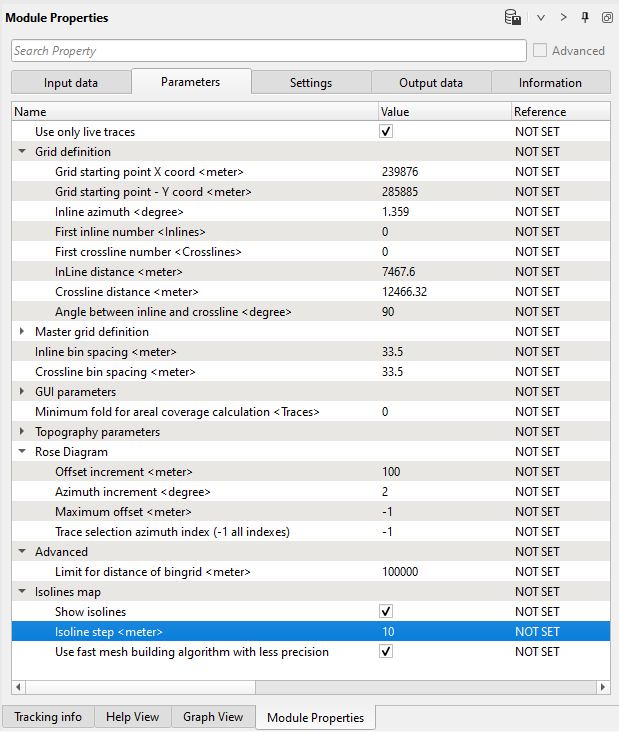
Next, set other parameters and execute the Binning 3D module:
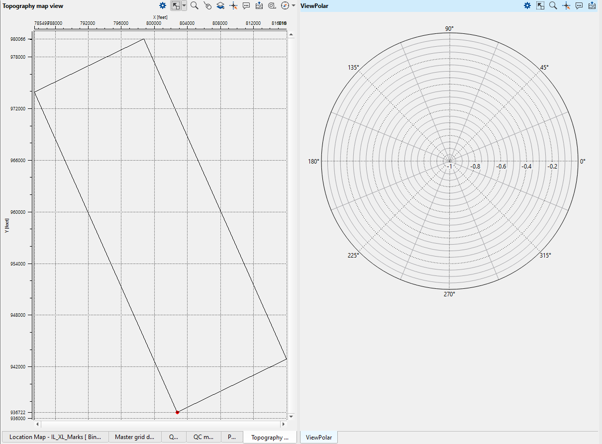
Fold map:
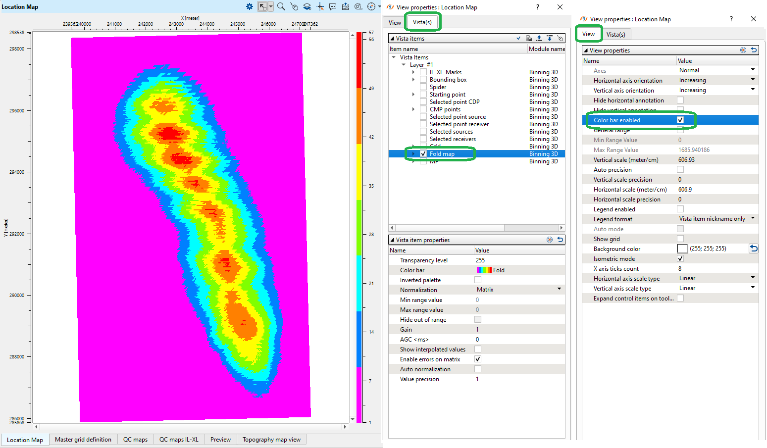
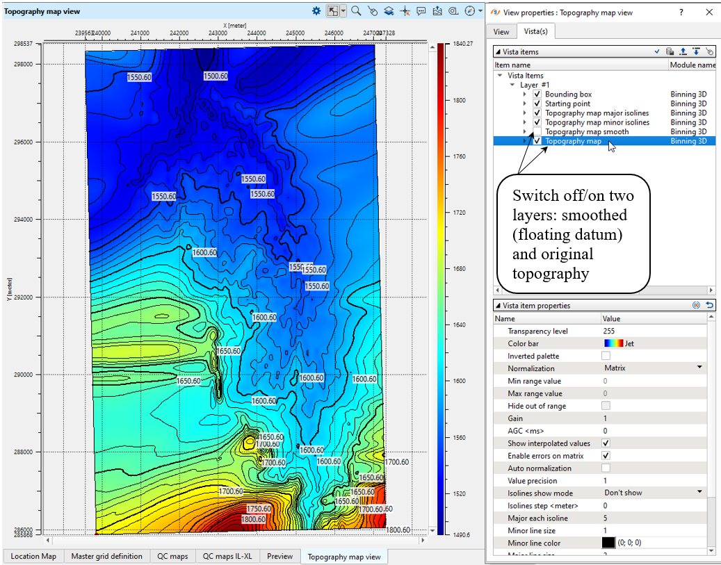
Make sure that you activated Show isoline option in the module's parameters (check previous step, parameters picture). Topography map contains smoothed topography which is a representation of the floating datum and it will be used for statics calculation:
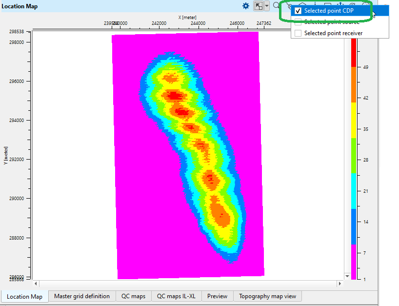
Check other visual windows like rose diagram and other. Then, return to the Location map and use interactive mode to see spider mode. Activate a mouse control mode to Selected point CDP:
Make zoom and click on any bin on the map (don't forget to switch on all layers in the View properties window - on the right side of the picture):
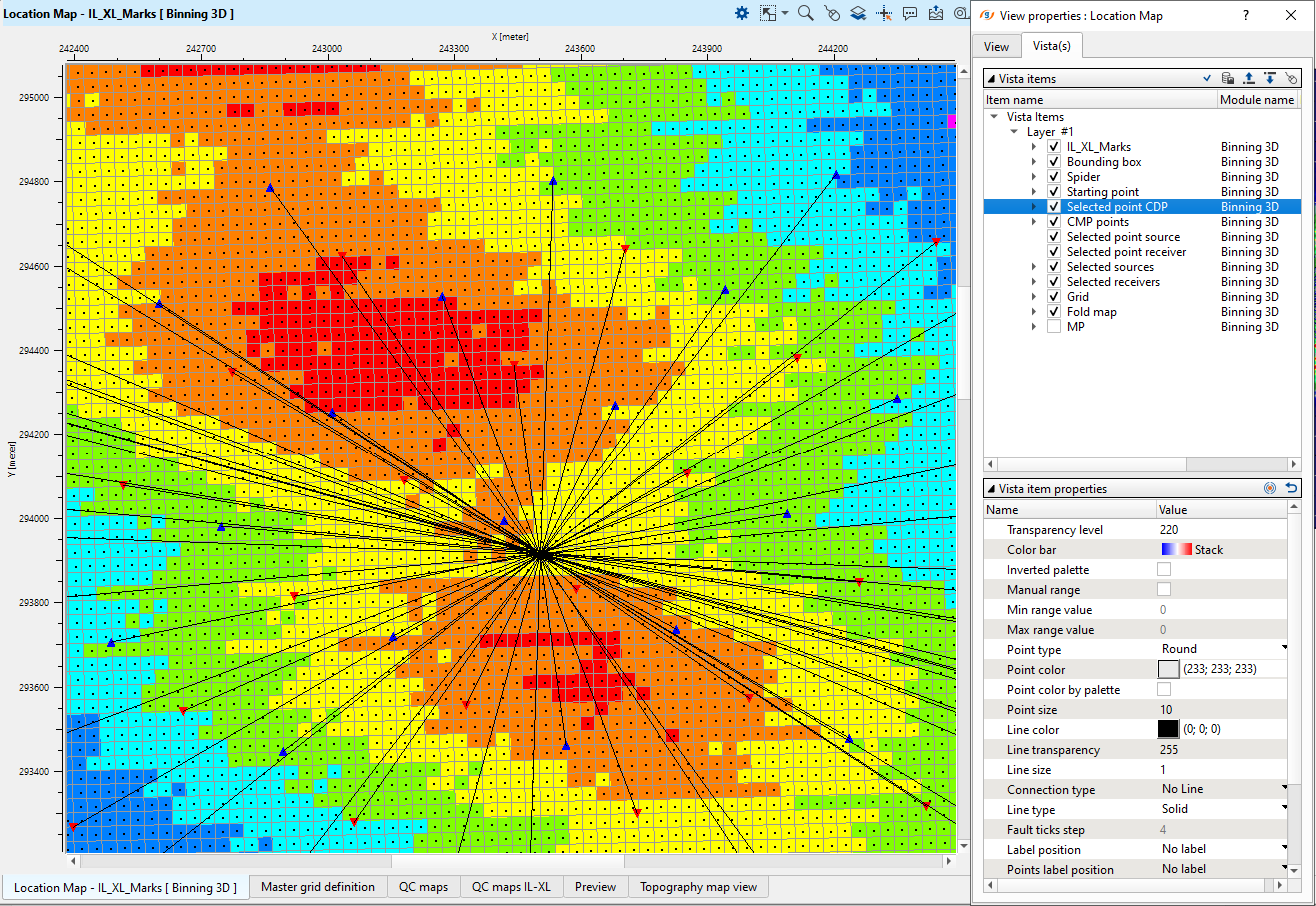
The binning is ready, all necessary traces headers were updated (BIN_X, BIN_Y, INLINE. CROSSLINE, ...). Check the output information from the Binning 3D module:
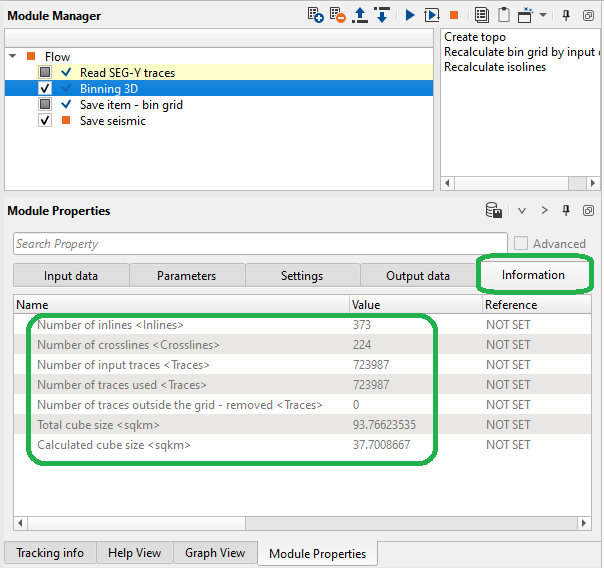
The main parameters of Binning 3D are described below:
| Use only live traces | By default checked. This will avoid any non-seismic traces get through to the next processing step. |
| Grid definition | This is where the user should provide the grid definition information |
| Grid Starting point X coord (feet) | Provide the grid starting X coordinate point. |
| Grid Starting point Y coord )feet) | Provide the grid starting Y coordinate point. |
| Inline azimuth (degree) | Specify the inline azimuth in degree. |
| First inline number (Inlines) | The user should provide the first inline number. By default it is 0. In case the user wants to match with the vintage data etc. they can provide as per the vintage data. |
| First crossline number (Crosslines) | Provide the starting Crossline number |
| Inline distance (feet) | It will automatically calculates the inline distance and the user doesn't have any input anything here. |
| Crossline distance (feet) | Same here as well. It will calculate the Crossline distance from the input data information. |
| Angle between inline and crossline | By default, 90 |
| Master grid definition | This is where the user should provide the 3 corner points information if it is available. Otherwise use the "Recalculate bin grid by input data" option. |
| First cornet point X - coordinate | Provide the fist corner point X-coordinate |
| First cornet point Y - coordinate | Provide the first corner point Y-coordinate |
| Inline direction corner point X-coordinate | Provide the coordinate point X-coordinate along the Inline direction |
| Inline direction corner point Y-coordinate | Provide the coordinate point Y-coordinate along the Inline direction |
| Crossline direction corner point X-coordinate | Provide the coordinate point X-coordinate along the Crossline direction |
| Crossline direction corner point Y-coordinate | Provide the coordinate point Y-coordinate along the Crossline direction |
| Number of Inlines add before corner point 1 | In case the user wants to extend the bin grid then specify the number of inlines to added before Corner point 1. |
| Number of Crosslines add before corner point 1 | Similar to Inlines, the user should add number of Crosslines to add before Corner point 1. |
| Number of Inlines add after corner point 4 | Specify the number of Inlines to be added after Corner point 4. |
| Number of Crosslines add after corner point 4 | Similar to Inlines, specify number of Crosslines to be added after Corner point 4. |
| Inline bin spacing | This is the actual bin grid size. Specify the Inline bin grid size. |
| Crossline bin spacing | Specify the crossline bin grid size. |
| GUI Parameters | These parameters doesn't play any role in actual binning processing but these are used for visualization only. |
| IL/XL GUI marks grid step | This parameter displays the Inlines/Crosslines at user defined interval. By default 25. It means, it will display every mark the Inline/Cross line numbers on the location map and others at 25 interval. |
| Minimum fold for real areal coverage calculation | By default Zero (0) |
| Topography parameters | Binning 3D creates the smoothed topography which acts as a Floating datum similar. |
| Interpolation method | Choose the available interpolation method for topography interpolation. By default, ABOS. |
| Elevation type | Choose the Source only, Receiver only or both Source and Receiver elevations to consider. |
| Smoothing distance (feet) | This parameter defines the topography smoothing distance. The higher the smoothing distance value, the more the topography smoothing. |
| Rose Diagram | These parameters are defined to display the directional distribution of the offset information wrt Azimuth. |
| Offset increment (feet) | Provide the offset increment value. Accordingly it will display the offset distribution in the rose diagram. |
| Azimuth increment (degree) | Based on the user defined azimuth increment, the rose diagram distribute the offset information at the user defined azimuth increment value. |
| Maximum offset (feet) | Provide the maximum offset to consider |
| Trace selection azimuth index | By default -1 which means it considers all the available traces. |
Advanced
| Limit for distance of bin grid (feet) |
| Isolines map | These parameters are basically for creating the contour maps or isoline maps. |
| Show isolines | By default Unchecked. If user checks this option, it will display the isolines however it slowdown the process a bit |
| Isoline step (feet) | Define the at interval the Isolines should be generated. In case Binning 3D is taking too much time, please pay attention to this parameter. |
| Use fast mesh building algorithm with less precision | By default checked. This option helps us to create the isolines map much faster. |
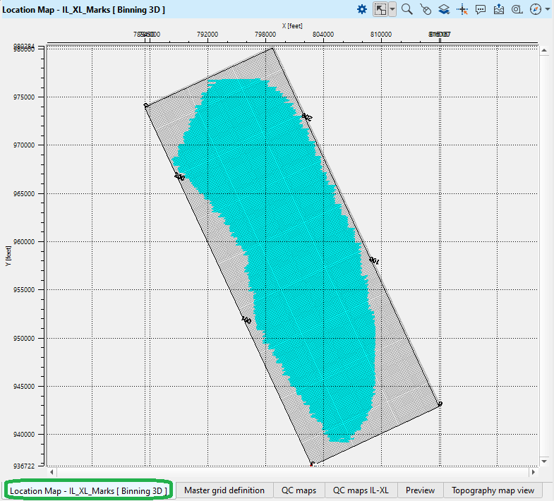
Provide all necessary module's parameters and launch the job, check results: Binning 3D gives various Vista items.
1. Location map with IL/XL marking
2. Master grid definition file
3. QC maps (Minimum and Maximum offset maps)
4. QC maps IL-XL (Check inline, crossline fold maps, min & max offsets, Topography maps etc)
5. Topography map (Both smoothed and unsmoothed)
6. Rose diagram with offset distribution.
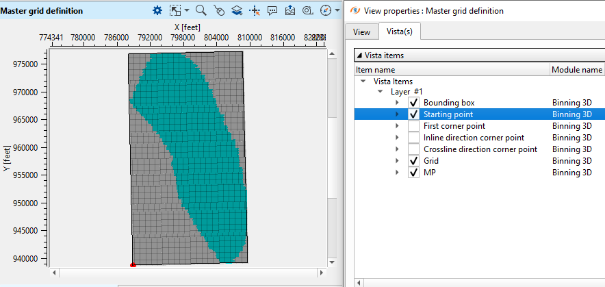
With respect to Master grid definition window, we can find each of the below mentioned by toggling on and off the Vista items one above or below in Show Properties window of Master grid definition.
1. Bin grid starting point (Red dot at the bottom left corner)
2. First cornet point (Same red dot at the bottom left corner)
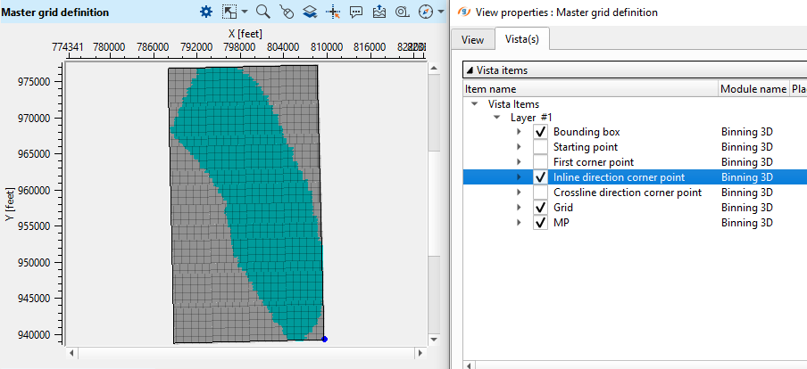
3. Inline direction corner point (Blue dot at the bottom right corner)
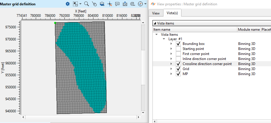
4. Crossline direction corner point (Green dot at the top left corner)
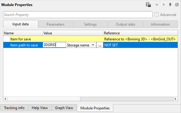
3) Save item - bin grid. Once the Binning 3D has been finished, we can save resulting Bin grid parameters for further processing steps (for example, migration). For that task g-Platform provides the Save item module, which is able to save bin grid into internal data base. Make all necessary connections in the Input data tab:
Input data:
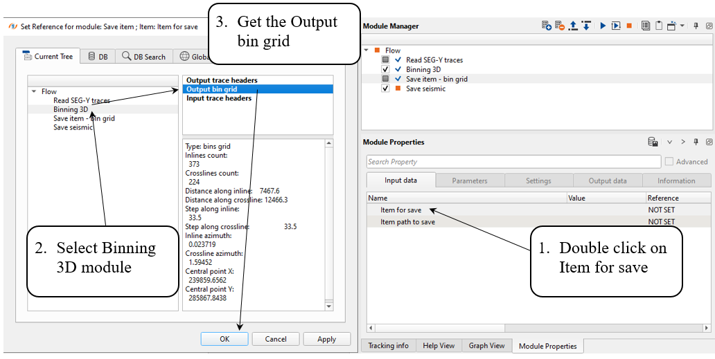
Define a name of the bin grid for data base and execute the module:
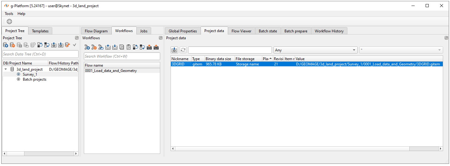
Check that grid was saved in DB, open the main window of g-Platform application and look at the Project data tab:
4) Save seismic. The last step is to save seismic data set with binning information into DB. First, we have to make two necessary input data connections:
Input data:
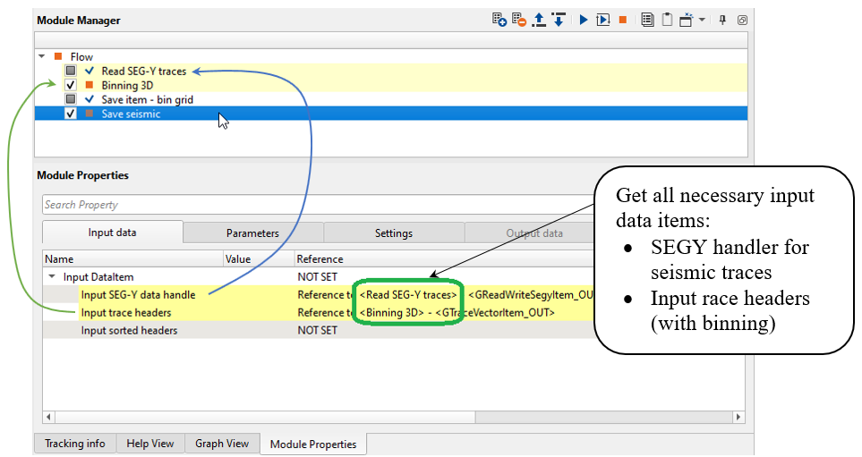
Define an output file name and activate Rewrite mode, execute the module.
Parameters:
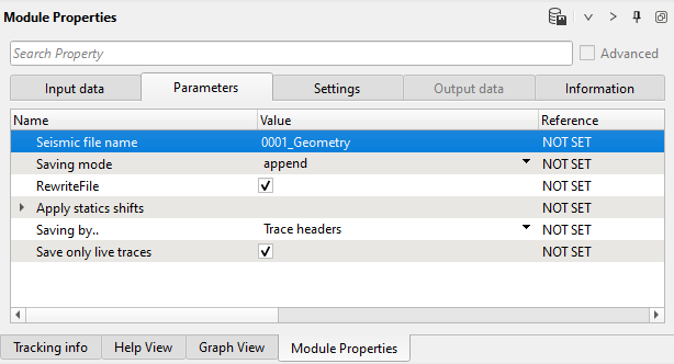
All seismic traces and headers with binning were saved!
------------------------------------------------------------------------------------------------------------------------------------------------------------------
![]() Be careful with the Saving mode = Append, in this case each time you execute module, each time it is adding seismic traces to the previous file, in other word 2 times run will lead to duplicates traces in output 0001_Iput_SEGY_3D file. To avoid the problem use RewriteFile mode.
Be careful with the Saving mode = Append, in this case each time you execute module, each time it is adding seismic traces to the previous file, in other word 2 times run will lead to duplicates traces in output 0001_Iput_SEGY_3D file. To avoid the problem use RewriteFile mode.
------------------------------------------------------------------------------------------------------------------------------------------------------------------
 If you have any questions, please send an e-mail to: support@geomage.com
![]() Load Geometry from SPS - Geomage g-Platform - YouTube
Load Geometry from SPS - Geomage g-Platform - YouTube
![]() Geometry Application - Geomage g-Platform - YouTube
Geometry Application - Geomage g-Platform - YouTube