 | REGULARIZATION & 5D INTERPOLATION |
|
<< Click to Display Table of Contents >> Navigation: Tutorials > Seismic Processing 3D LAND >
|
Seismic data acquired in the field is not regular in terms of space between offset classes and existing near and far offsets. The process is called regularization, which is required to perform prior to the migration step, as well as for getting better imaging in case of poor fold and offset survey coverage. Please keep in mind that the regularization and interpolation are not an alternative or replacement of the field acquisition. It is a tool to regularize the data followed by filling the missing data using the interpolation. There are various methods to regularize the 2D/3D data and interpolate the missing data.
Why do we regularize, interpolate the data and what is a 5D means?
A field data acquired in various conditions. In some cases, it is very difficult to acquire the data in a regularized fashion. That leads to irregular grid and data gaps. With the regularization and interpolation, we can fill the gaps and achieve a good regularized data within g-Platform system.
An input binned data set consists of inline, crossline, offset, time and azimuth information. In other words, source-x, source-y, receiver-x, receiver-y and time.
The advantages of interpolation data are:
1. Better signal to noise ratio;
2. Improving the overall image quality;
3. Better offset, azimuth distribution.
In our tutorial, we are going to discuss the regularization of the data by using different regularization methods. The process is as described below:
1. Read the input data: should be performed all noise steps and multiple attenuation, statics applied, non-NMO corrections, because for regularization it is not required to have NMO corrected gathers, but for 5D interpolation we provide the velocity model and it will apply forward and reverse NMO correction. Final output gathers from 5D interpolation are no-NMO gathers;
2. Apply binning procedure (just to make sure we are having a right bin grid information). If you sure, you can skip this step, but need to load the bin grid by using Load item module and provide the previously saved bin grid library item;
3. Sort the data by INLINE, CROSSLINE , ABS OFFSET order;
4. Provide the velocity model which was previously saved by using Load item or via creating one by Create velocity model module;
5. Choose the regularization method from the available options. Here, we input the original bin grid and regularize the data using the selected regularization scheme. Followed by binning the regularized trace headers. These trace headers are now regularized and can be used an input to the 5D interpolation.
Pay attention that current chapter explains a few different regularization methods (spiral, polar, virtual SC , ...), so you just need to test all of them and decide which one to use.
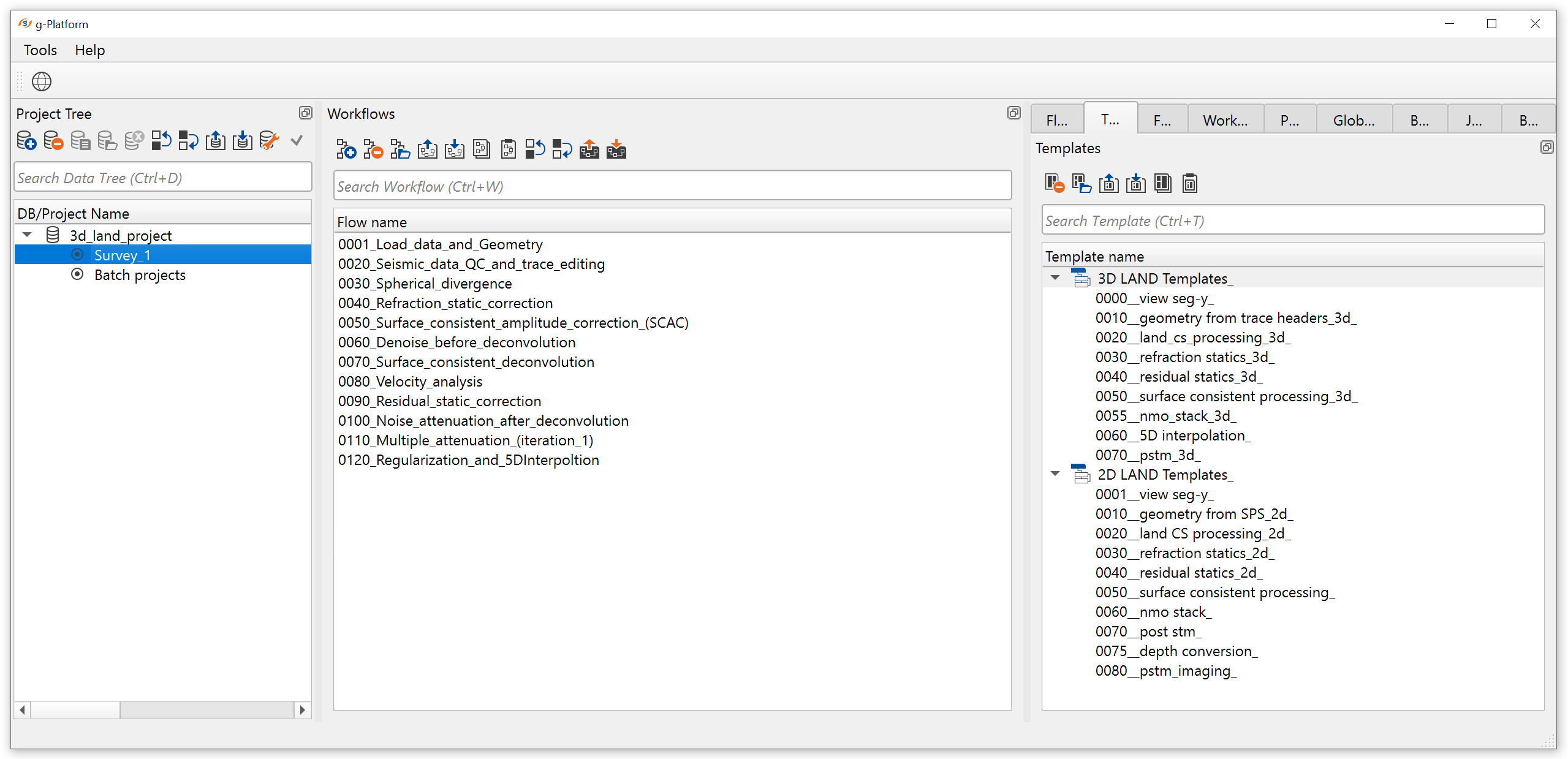
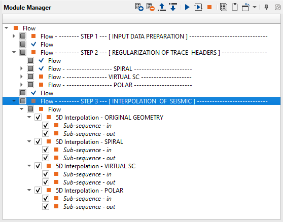
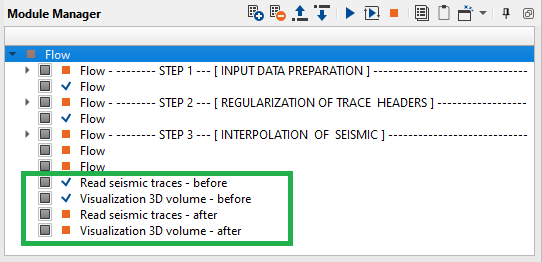
Create a workflow 0120_Regularization_and_5DInterpolation as shown below:
The workflow is spitted into 3 parts:
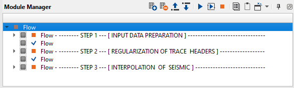
STEP 1: INPUT DATA PREPARATION
Add all necessary modules to this part of the workflow:
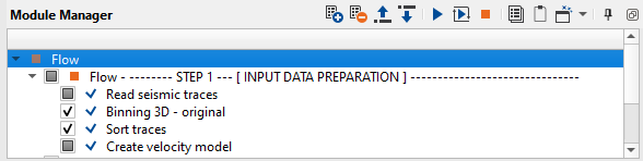
1. Read seismic traces
2. Binning 3D - original
3. Sort traces
4. Create velocity model
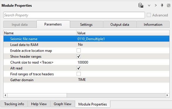
1) Read seismic traces: load 0110_Demultiple1 seismic data set.
Parameters:
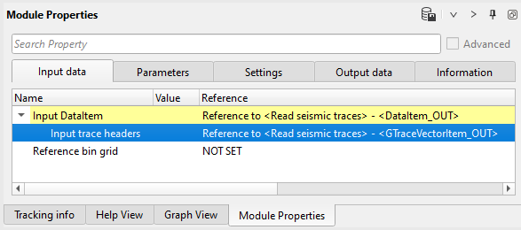
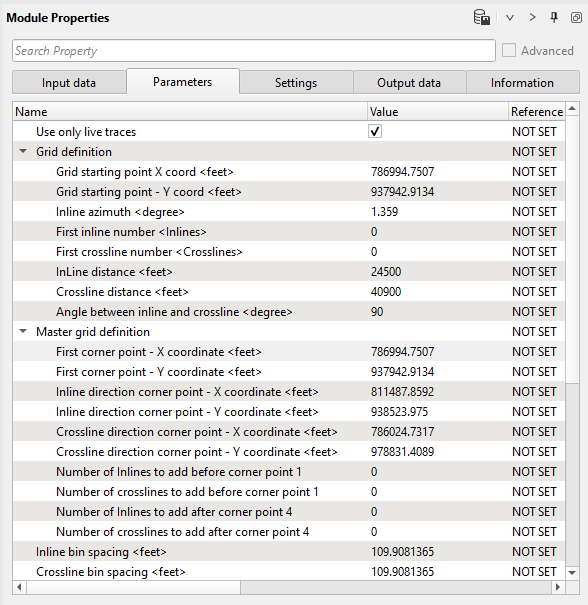
2) Binning 3D: Do the binning 3D, you can copy-> paste this module from the geometry workflow. We will use 3D grid in regularization module and fold map for QC. Parameters are the same as were in geometry binning, so we just need to connect input trace headers from read seismic traces:
Input data:
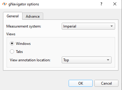
Reminder: we are using imperial system:
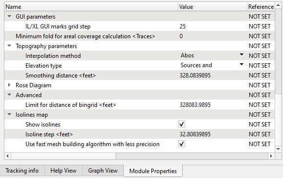
Parameters:
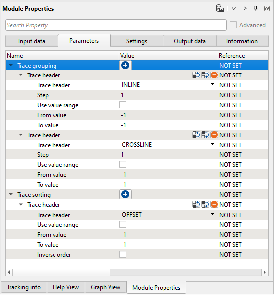
3) Sort traces: Sort the data by inline, crossline as Trace Grouping - Abs Offset as Trace sorting:
Parameters:
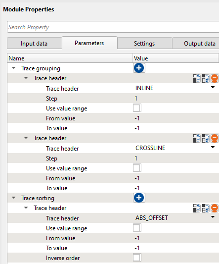
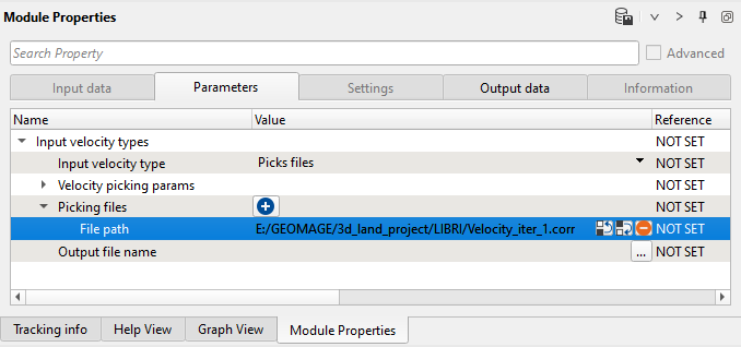
4) Create Velocity model: Create the velocity model by selecting the Input velocity type as Picks file. Next click on ![]() icon and define a path and file name of the the input velocity file:
icon and define a path and file name of the the input velocity file:
Parameters:
These are the main input data requirements for data regularization. After that, we can choose the preferred regularization methods/schemes and prepare the data for the next step i.e. interpolation. The workflow for regularizing the data by using any of the regularization methods/schemes is describes below.
STEP 2: REGULARIZATION OF TRACE HEADERS
We are going to test 3 regularization algorithms: Spiral, Virtual SC and Polar:
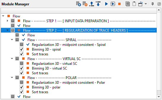
Each scheme contains 3 modules:
1. Regularization 3D - mid point consistent - Spiral or Regularization 3D - mid point consistent - Polar or Regularization 3D - mid point consistent - Virtual SC or any other;
2. Binning 3D - Binning the output trace headers of regularization 3D module;
3. Sort traces - Sorting the output trace headers of Binning 3D module.
S P I R A L:
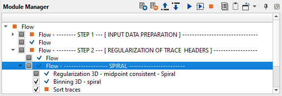
1. Regularization 3D - midpoint consistent - Spiral
2. Binning 3D - spiral
3. Sort traces
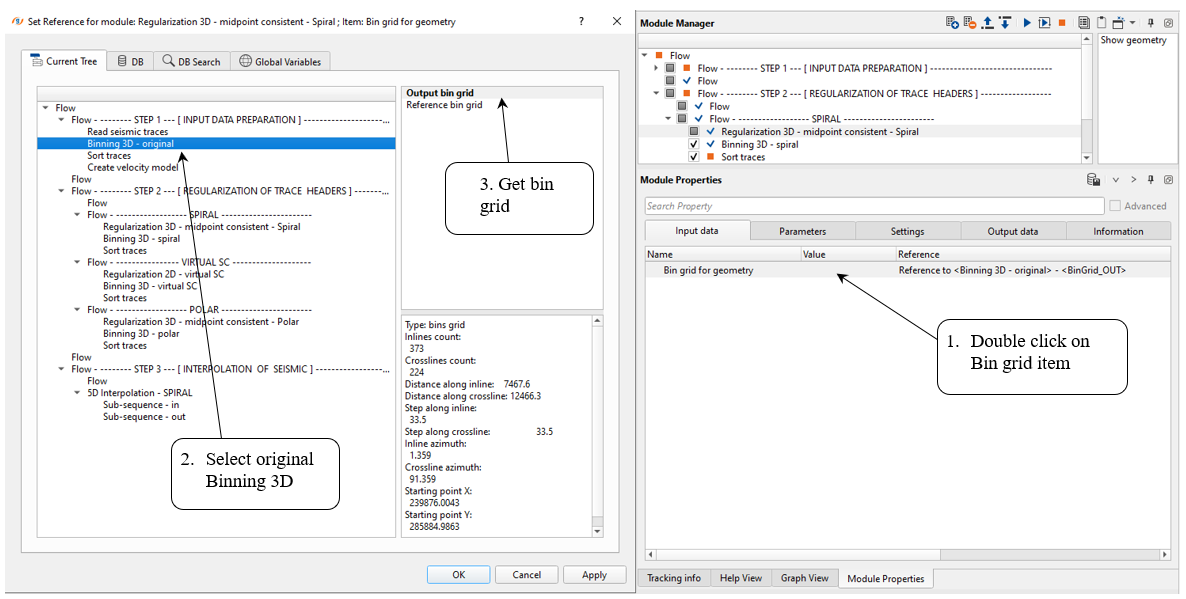
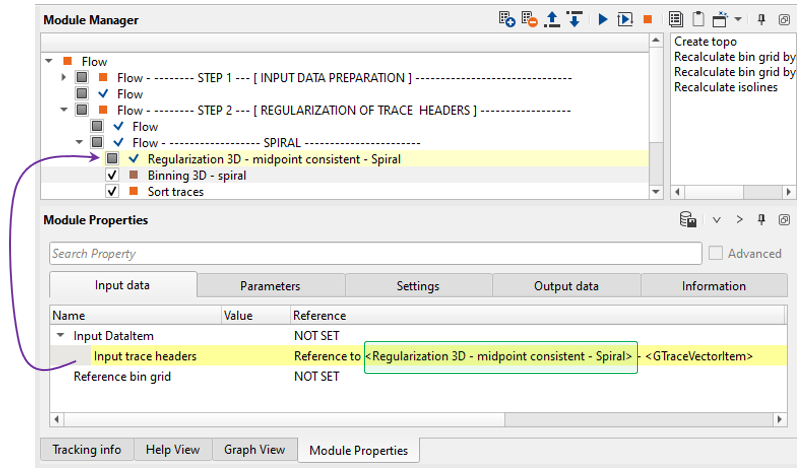
1) Regularization 3D - midpoint consistent - Spiral: Trace header regularization withing Spiral algorithm.
This is one of the regularization 3D modules available among others. Here we need to make the connections/reference of Bin grid for geometry to Binning 3D module output bin grid.
Input data:
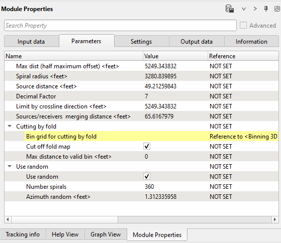
Parameters:
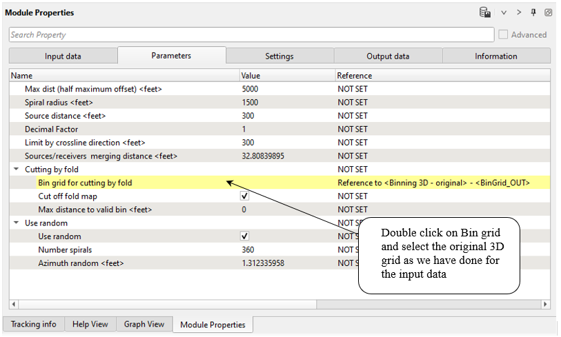
Parametrization:
Max dist (half maximum offset)
This parameter takes the offset information. Provide the half of the maximum offset.
Spiral radius
This parameter defines how much spiral radius should be provided. The bigger the radius the more coverage. It doesn't guarantee that the bigger number works better.
Source distance
Define the distance between adjacent sources.
Decimal factor
It will decimate the number of sources and receivers by the user defined number.
Limit by crossline direction
Define the bound limitation via crossline direction in feet/meters.
Sources/receivers merging distance
Minimum distance between two adjacent sources/receivers. If the adjacent sources/receivers are falling below this value, they will be merged together to make a single source/receiver.
Cutting by fold:
We can limit/control the regularization by means of fold of the input data. Beyond input fold, there will not be any regularization.
Bin grid for cutting by fold
Provide the input bin grid.
Cut off fold map
By default, checked. It will cut off any regularization outside the input fold map.
Max distance to valid bin
Maximum distance for valid bin cell, by default it is zero.
Use random:
Use random
Check box option for using random spiral distribution.
Number spirals
Amount of spirals / circle coverage.
Azimuth random
Azimuth value in radians.
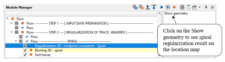
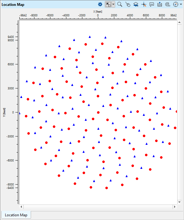
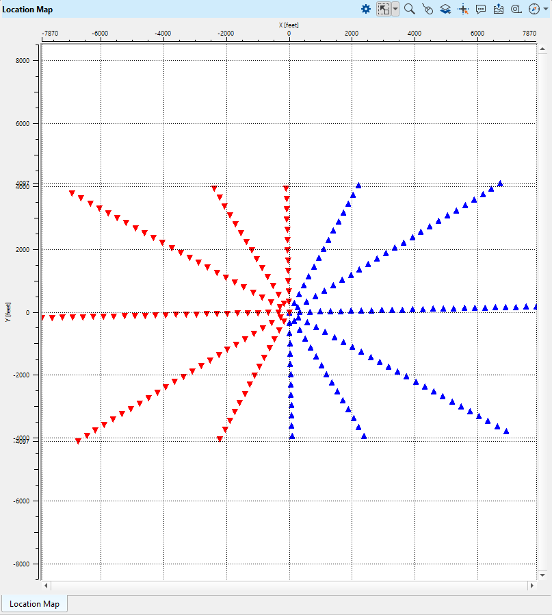
We can QC the parameters by looking at the Location map Vista item of the Regularization 3D - mid point consistent - Spiral module. To QC the parameters, we should click on the Show geometry option in the action menu:
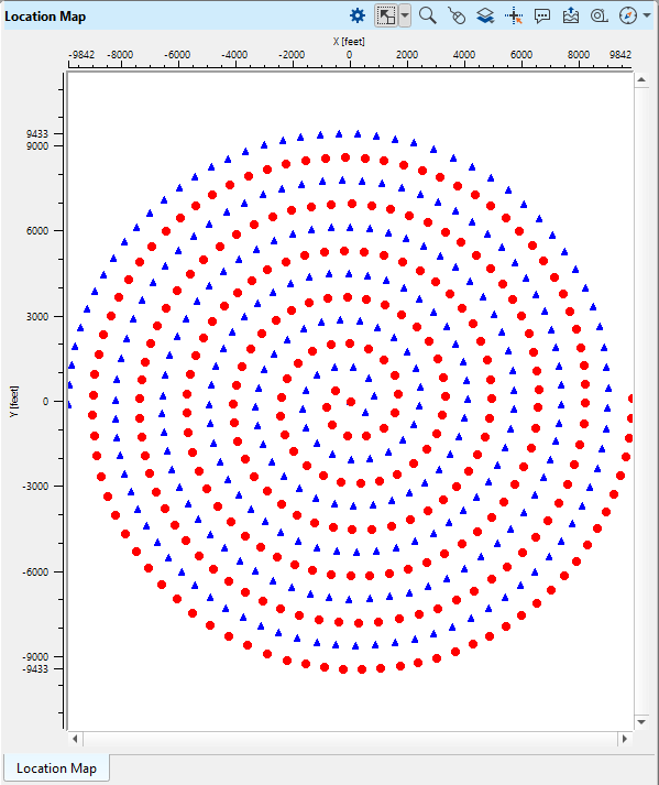
In the below images, we have one location map with Decimal factor as 1 and the other one as 3. Similarly, we can change the source distance, spiral radius and other parameters and visualize before proceeding further:
Decimal factor = 1 Decimal factor = 3
Once the parametrization is finalized, just execute the Regularization 3D - mid point consistent - Spiral module (double click on the module).
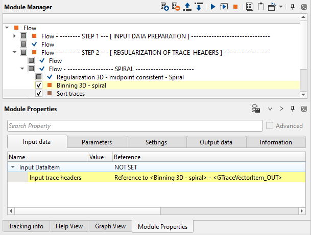
2) Binning 3D - spiral: Get the latest trace headers of the Regularization 3D - mid point consistent - Spiral module as input to the Binning 3D module. Other binning parameters are same as the input data (so we just can copy->past Binning 3D module):
Input data:
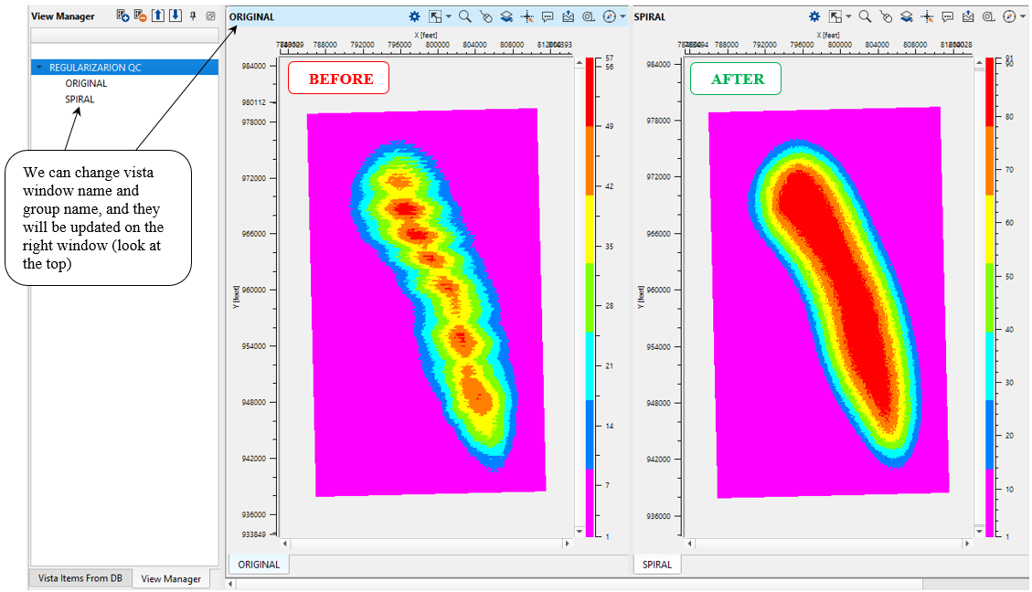
Next, display 2 location maps from the original and regularized Binning 3D. Switch off the all unnecessary vista items from the View properties of both the Binning 3D location maps (original and regularized). Also switch on the Color bar enabled option and select Fold map:
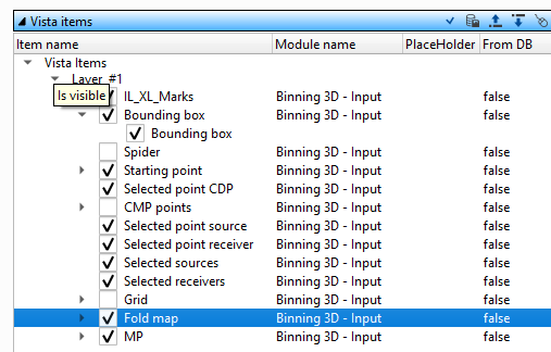
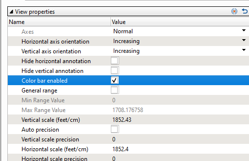
In the below image, we have fold map from the input data on the left side, fold map from the regularized 3D - mid point consistent - Spiral on the right. As we mentioned earlier, we can test regularization on fly (fast process) with different parameters to get the optimum results.
3) Sort traces: Now we need to sort the traces for further 5D interpolation process. Output trace headers of the Binning 3D - spiral module should be the input trace headers for Sort traces module.
Input data:
Parameters:
This test was done and now we can try other regularization algorithms.
V I R T U A L S C:
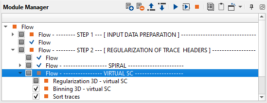
1. Regularization 3D - midpoint consistent - Spiral
2. Binning 3D - virtual SC
3. Sort traces
1) Regularization 3D - Virtual SC: Trace header regularization withing Spiral algorithm.
This is another one of the regularization 3D modules available among others. Here we need to make the connections/reference of Bin grid for geometry to Binning 3D module output bin grid. The main idea is the same as it was on the previous test: regularization, binning, sorting.
Parameters:
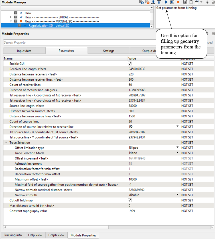
Parameters:
Enable GUI
Receiver line length
Specify the receiver line length.
Distance between receivers
Provide the distance between two adjacent receivers.
Distance between receiver lines
This is parameter is related to the distance between two receiver lines.
Count of receiver lines
Specify the total number of receiver lines.
Direction of receiver line
Define the receiver line direction i.e. usually the inline azimuth direction.
1st receiver line X
Coordinate of 1st receiver - provide the 1st receiver point X coordinate.
1st receiver line Y
Coordinate of 1st receiver - provide the 1st receiver point Y coordinate.
Source line length
Specify the line length of the source.
Distance between sources
Provide the distance between two adjacent sources.
Distance between source lines
Define the distance between two source lines.
Count of source lines
Specify the total number of source lines.
Direction of source line relative to receiver line
This is the angle between source and receiver line usually 90 degrees.
1st source line X - coordinate of 1st source
Provide the 1st source point X coordinate.
1st source line Y - coordinate of 1st source
Provide the 1st source point Y coordinate.
Trace selection:
Offset limitation type
Choose the options available from the drop down menu. This is basically to limit the offset based on the type of trace selection. By default, we have Ellipse.
Trace selection mode
None by default. In case the user selects By Offset or By Offset/Azimuth option then the those parameters will be activated otherwise they will be disable with Trace selection mode as None.
Offset increment
In case the Trace selection mode is selected as By offset then provide the offset increment step size.
Azimuth increment
If Azimuth is selected as a Trace selection mode then provide the Azimuth increment value.
Decimation factor for min offset
By default 1.
Decimation factor for max offset
By default 1.
Maximum offset
Define the maximum offset should be consider in the virtual geometry.
Maximal fold of source gather
Narrow azimuth maximal distance
Narrow azimuth
By default disable.
Cut off fold map
The user can limit/control the regularization by means of fold of the input data. Beyond input fold, there will not be any regularization/
Maximum distance to valid bin
By default Zero.
Constant topography value
Provide the constant topography value in case the user wants to change the topography value. By default, -999/
Once the parameters are set, execute the Regularization 3D - mid point consistent - Virtual SC. Next, do the same with binning and sorting.
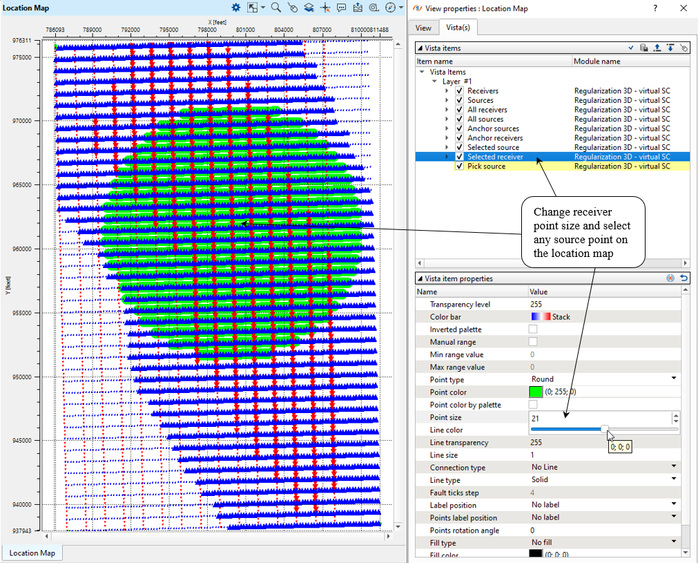
Open vista windows - Location map:
2) Binning 3D - virtual SC: the same as was before, just need to change input data traces headers.
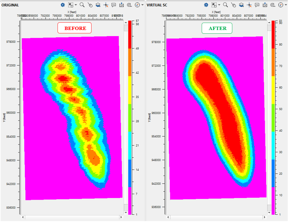
Now we can compare fold maps (from binning 3D modules): original vs Virtual SC regularization. The resultant display should be like this as shown below.
3) Sort traces: the same as was before, just need to change input data traces headers.
P O L A R:
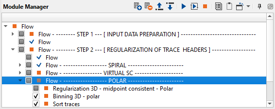
1. Regularization 3D - midpoint consistent - Polar
2. Binning 3D - polar
3. Sort traces
1) Regularization 3D - mid point consistent - Polar
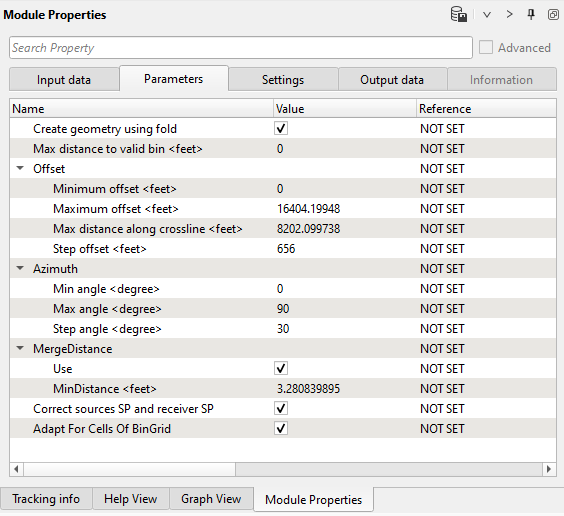
Parameters:
Create geometry using fold
By default check. It will use the input geometry fold information and accordingly create the geometry.
Max distance to valid bin
By default Zero.
Offset
Define the required offset information.
Minimum offset
Specify the minimum offset.
Maximum offset
Specify the maximum offset.
Max distance along crossline
Provide the maximum distance along the crossline.
Step offset
Specify the offset step size.
Azimuth
Min angle
Provide minimum azimuth angle.
Max angle
Provide maximum azimuth angle.
Step angle
Provide the angle step size.
Merge distance
Use
By default checked. It means it will merge the adjacent source/receiver if it fulfill the user defined minimum distance.
Min distance
Specify the minimum distance between two source/receivers to merge.
Correct sources SP and receiver SP
By default checked. It will correct the source and receiver SPs if there exists any errors.
Adapt for cells of bin grid
By default Checked.
Open location map and test parameters.
2) Binning 3D - virtual SC: the same as was before, just need to change input data traces headers.
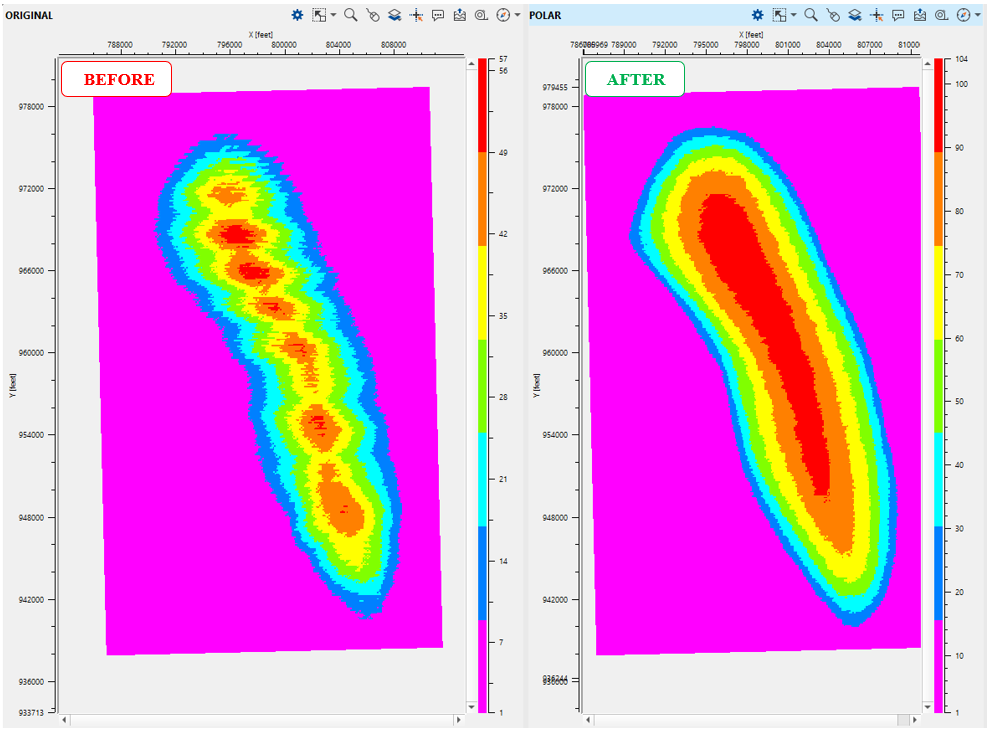
Now we can compare fold maps (from binning 3D modules): original vs polar regularization. The resultant display should be like this as shown below.
3) Sort traces: the same as was before, just need to change input data traces headers.
In the same way, we can try the other available regularization schemes. So,we already have been prepared the data for next stage which is 5D interpolation (5DI). We take the output trace headers from these regularization 3D modules and make connection as input trace headers.
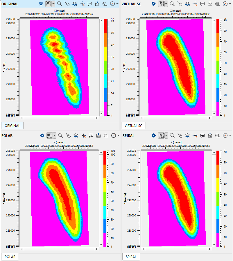
Now we can compare all fold maps:
STEP 3: INTERPOLATION OF SEISMIC
The third part of the workflow is seismic trace interpolation. There are four 5D Interpolation modules: one original geometry and three regularizations: spiral, virtual SC and polar:
5D Interpolation: We do 5DI in Tau-P domain where it is required to provide the inline and cross line aperture for the bin selection area (interpolation and extrapolation). Within the provided aperture, the algorithm will get the source and receiver combinations and perform the interpolation of inline, crossline, offset, azimuth and frequency. If there are not enough source-receiver combinations are available then there will be data gap which can't be filled. However, we can increase/decrease the inline and crossline aperture size to minimize the data gaps.
In this section, we are going to discuss 5D interpolation step and look at the results of the original input data and interpolated using regularized grid.
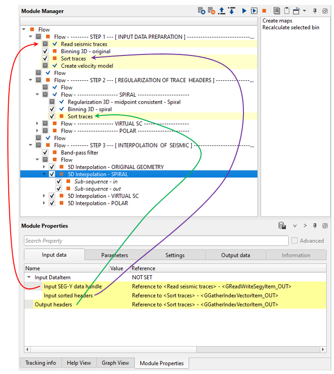
Define the input and output parameters of 5D Interpolation - SPIRAL. For data interpolation, we consider the original input data gathers as input data and the output trace headers will be from one of the regularization 3D schemes.
Input data:
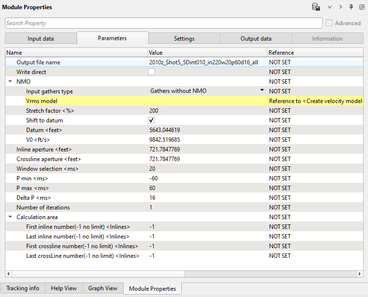
Parameters:
Pay attention that we use Output headers input data item from the original sorting (Sort traces module).
Output file
Specify the output file name.
Write direct
By default checked.
NMO:
Input gather type
By default NMO Gathers. If the input gathers are NMO gathers, we don't need to provide the Vrms model. If the Input gather type is Gathers without NMO, then provide the Vrms model by connecting to Create velocity model module.
Stretch factor %
Specify NMO stretch factor in %.
Shift to datum
By default checked. If we want to shift the data to final datum, provide the datum value in the next parameter.
Datum
Provide the datum value.
V0
Provide the near surface or replacement velocity.
Inline aperture
Specify the aperture size in inline direction for doing the interpolation.
Crossline aperture
Specify the cross line aperture.
Window size
Define the window size for vertical interpolation.
P min
Provide the minimum P value.
P max
Provide the maximum P value.
Delta P
Define the delta P.
Number of iterations
Specify the number of iterations to perform.
Calculation area
This is where we can specify a particular inline/cross line for testing the parameters. Besides, without specifying these parameters also we can perform the interpolation and visually QC the results. There is no need to specify these details when the process is executing: the 5DI for the entire volume.
First inline number
Specify the first inline number.
Last inline number
Specify the last inline number.
First crossline number
Specify the first crossline number.
Last crossline number
Specify the last crossline number.
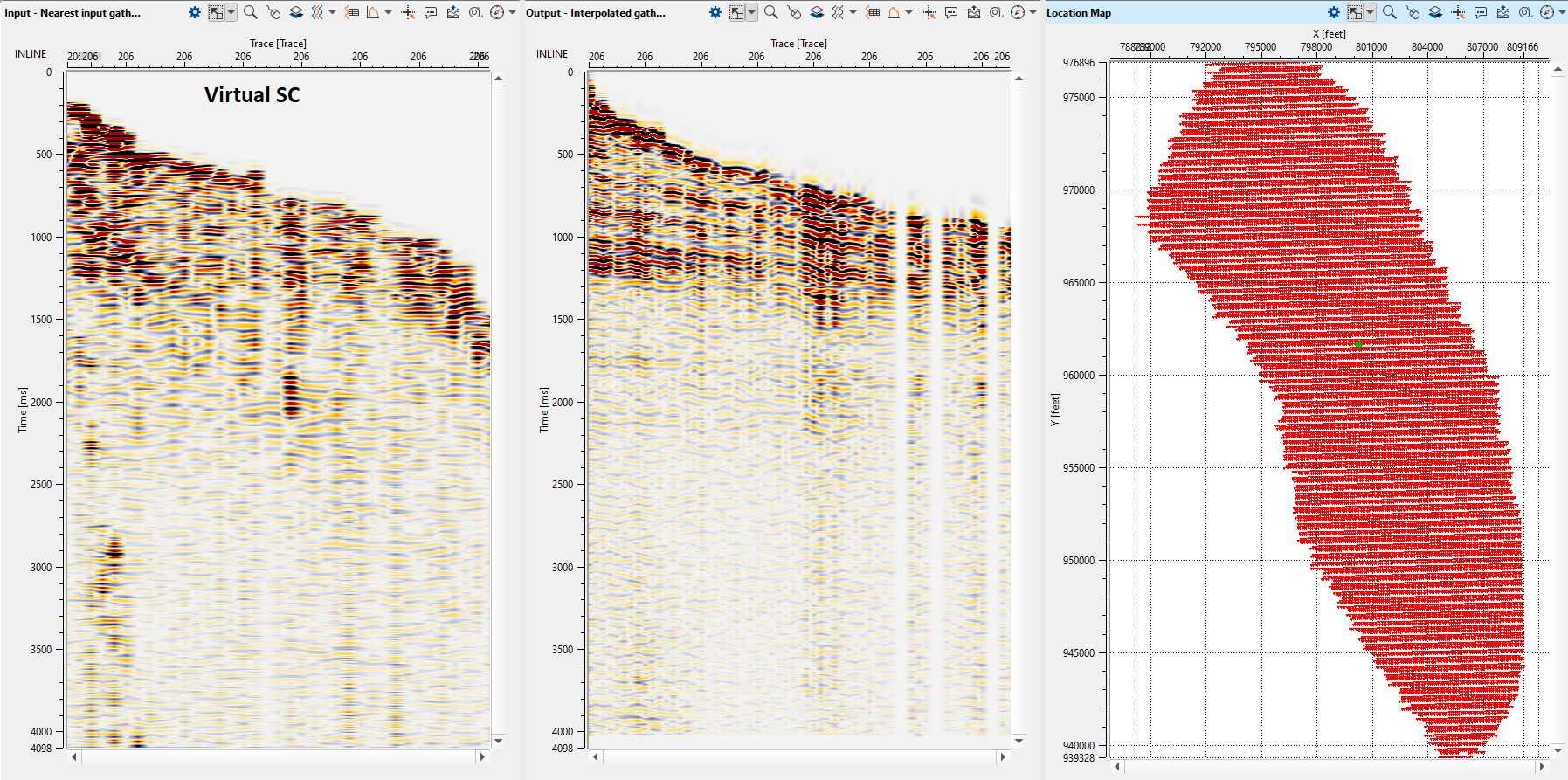
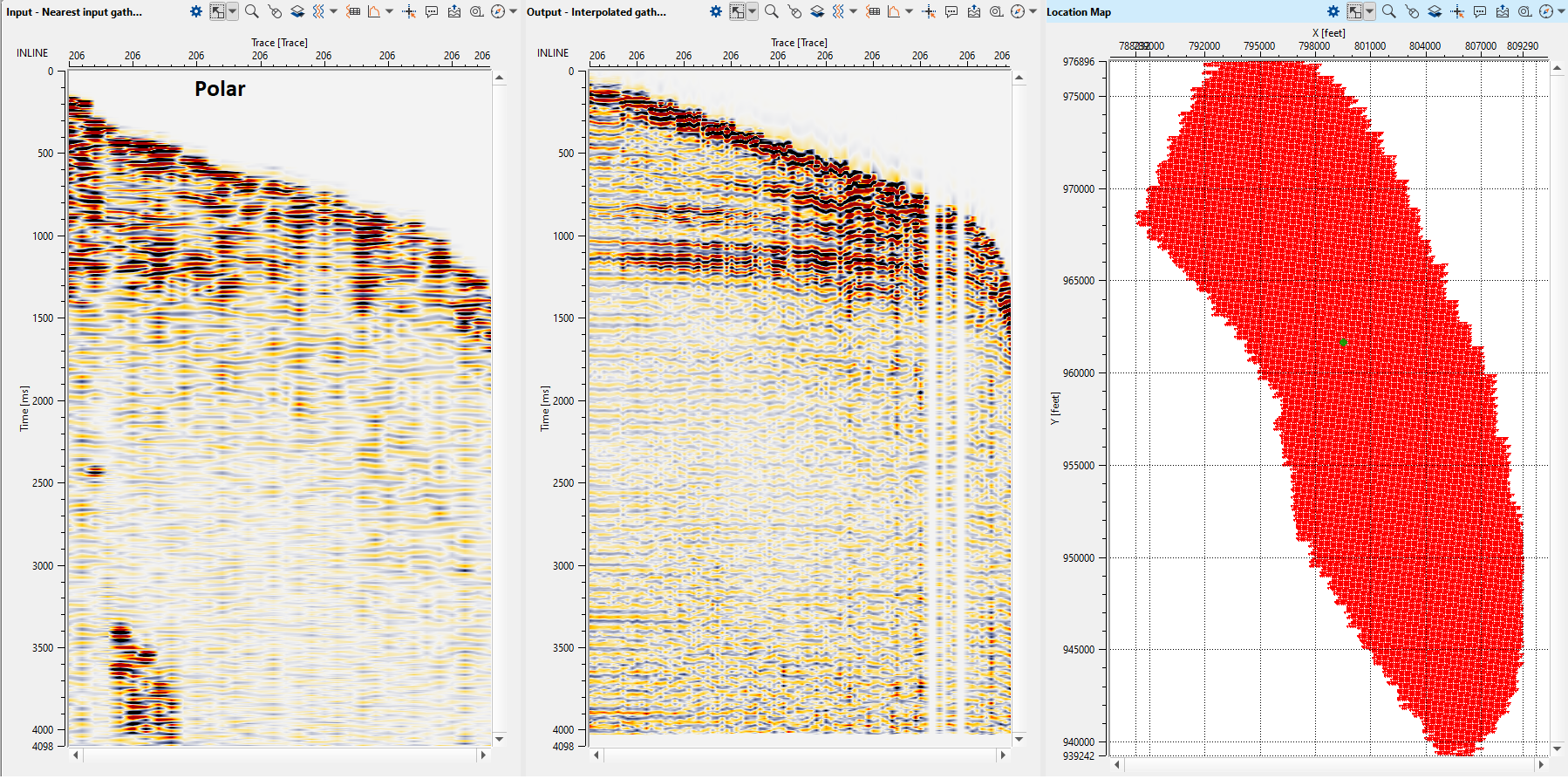
When the parametrization is ready, display the Vista items of 5D Interpolation. After launching, it will display everything empty including Location map. To view the location map, we should click on Create maps option in the action menu of the 5D Interpolation module followed by clicking Recalculate selected bin. This will display the location map along with the Input and Output gathers.
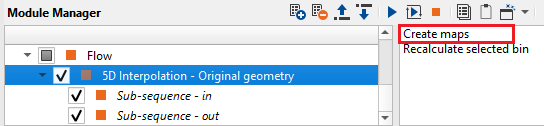
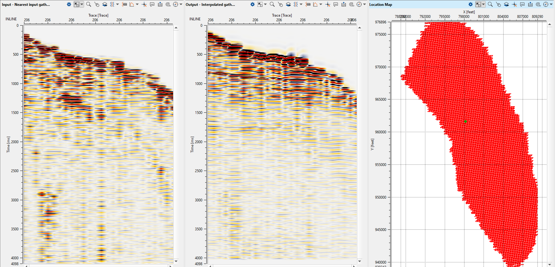
In the above image, we can see a green dot on the location map. It is the current selected bin and it is showing the resultant gather before and after 5D interpolation. We can select any random location on the location map and click the Recalculate selected bin and wait for the output to be displayed.
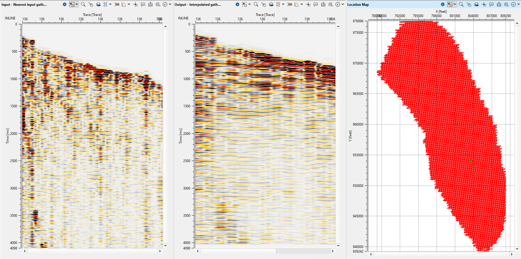
In the same way, we can check the 5DI results using different regularization schemes and compare which one is the best for further processing . In the following examples, we are showing the output gathers of Spiral, Virtual SC and Polar regularization schemes.
Please make a note that we should connect/reference the Sort traces to Sort traces of the respective regularization schemes. In case of Regularization 3D - mid point consistent - Spiral, the output sorted traces should be connected to the input sort traces of the 5D interpolation module.
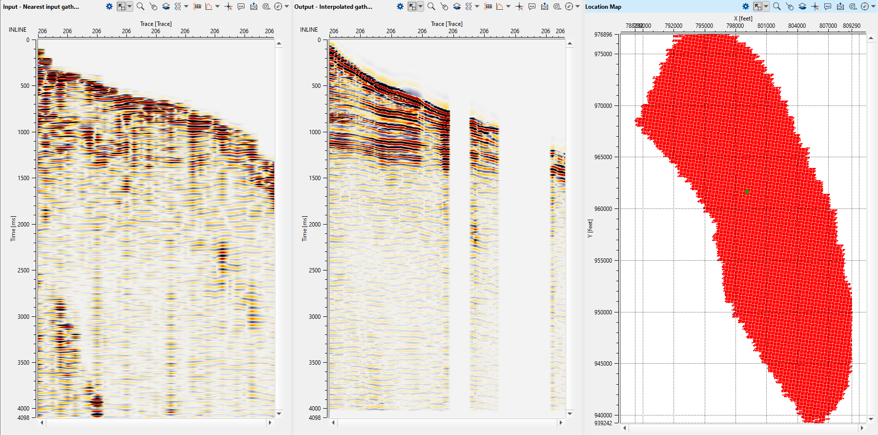
We can see some data gaps in the output. To fill them, we can test different inline and crossline aperture values and Recalculate selected bin, then check the results.
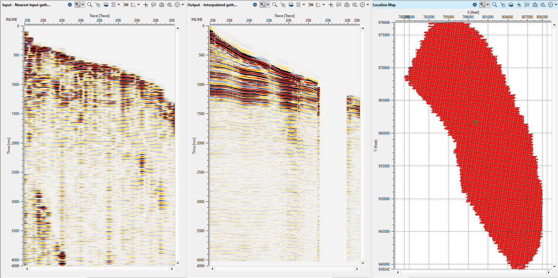
Likewise for other regularization schemes and get the output results.
You can select regularization algorithms and its parameters as you wish. We used spiral mode with the following parameters:
Parameters:
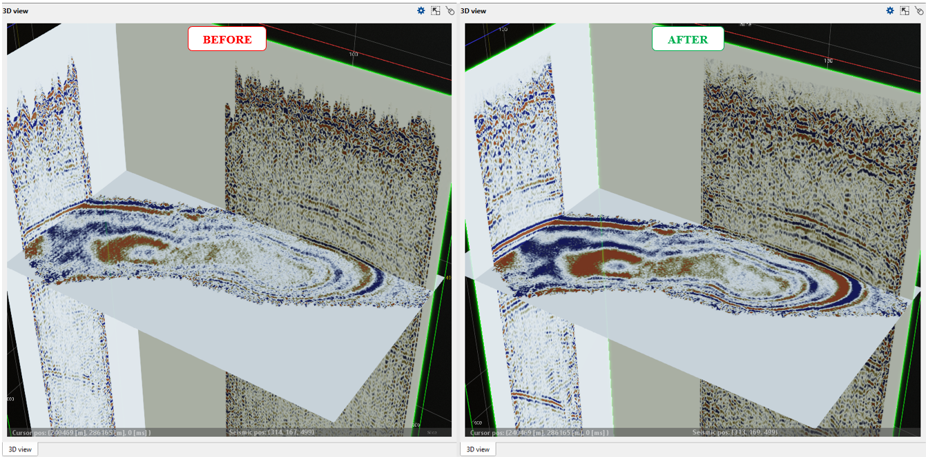
Execute interpolation for the entire data set, create stack cubes before and after regularization (you may use separated workflow for stack creation, we will skip them in the current chapter). Load them and use Visualization 3D module for time slice comparison:
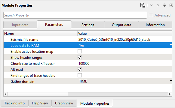
Parameters:
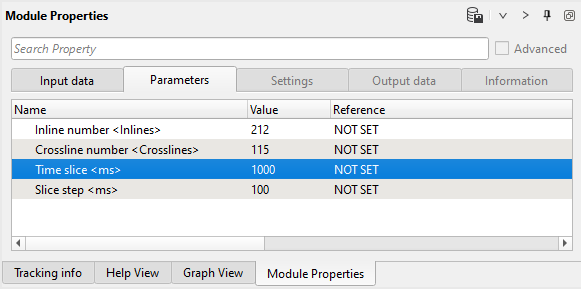
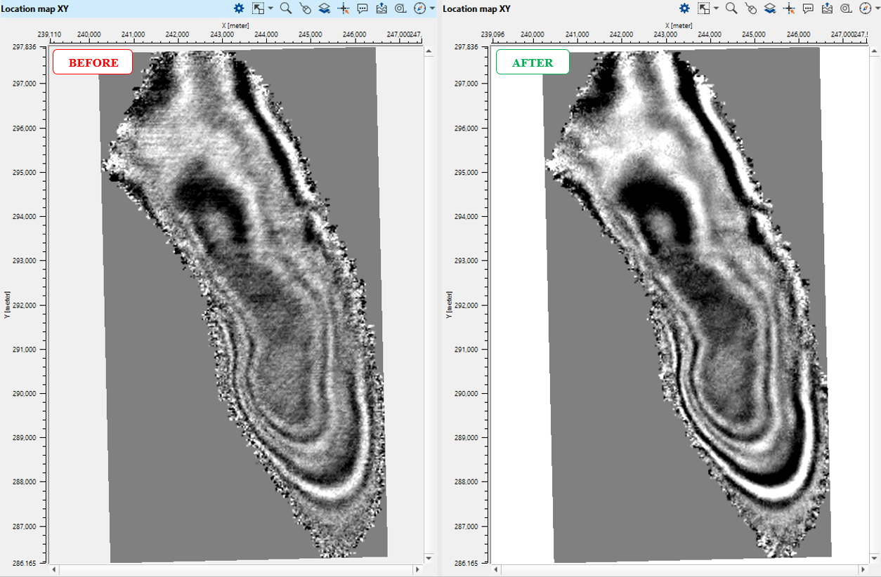
Time slice 1000 ms after regularization:
Compare time slices (1000ms) before and after:
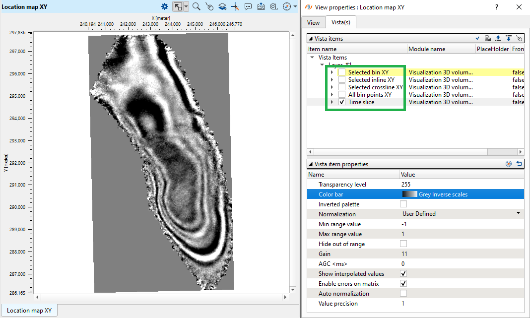
Configure location map view:

And compare two crosslines:
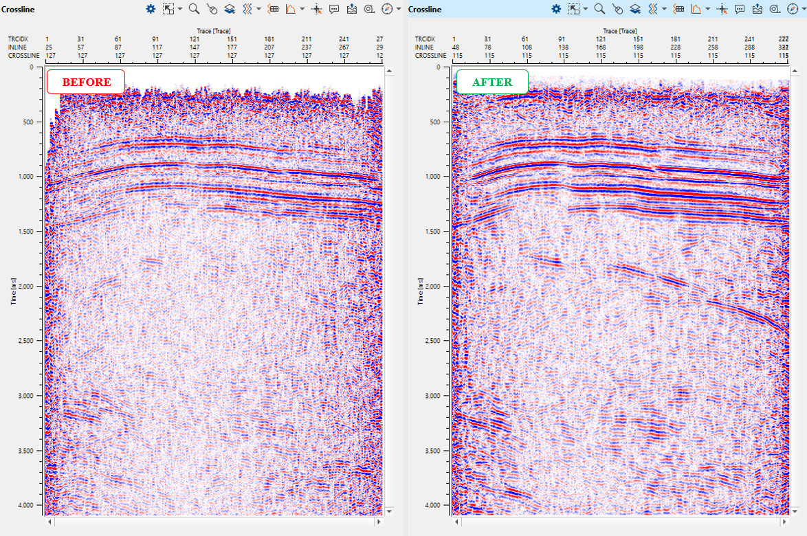
Use 3D view windows for QC:
Control actions:
•Left mouse button for selection inline/crossline/slice;
•Right mouse button + control for spinning;
•Right mouse button + shift for moving (the entire cube, left/right/up/down).
 If you have any questions, please send an e-mail to: support@geomage.com