Creating 3D volume from multiple 2D lines
![]()
![]()
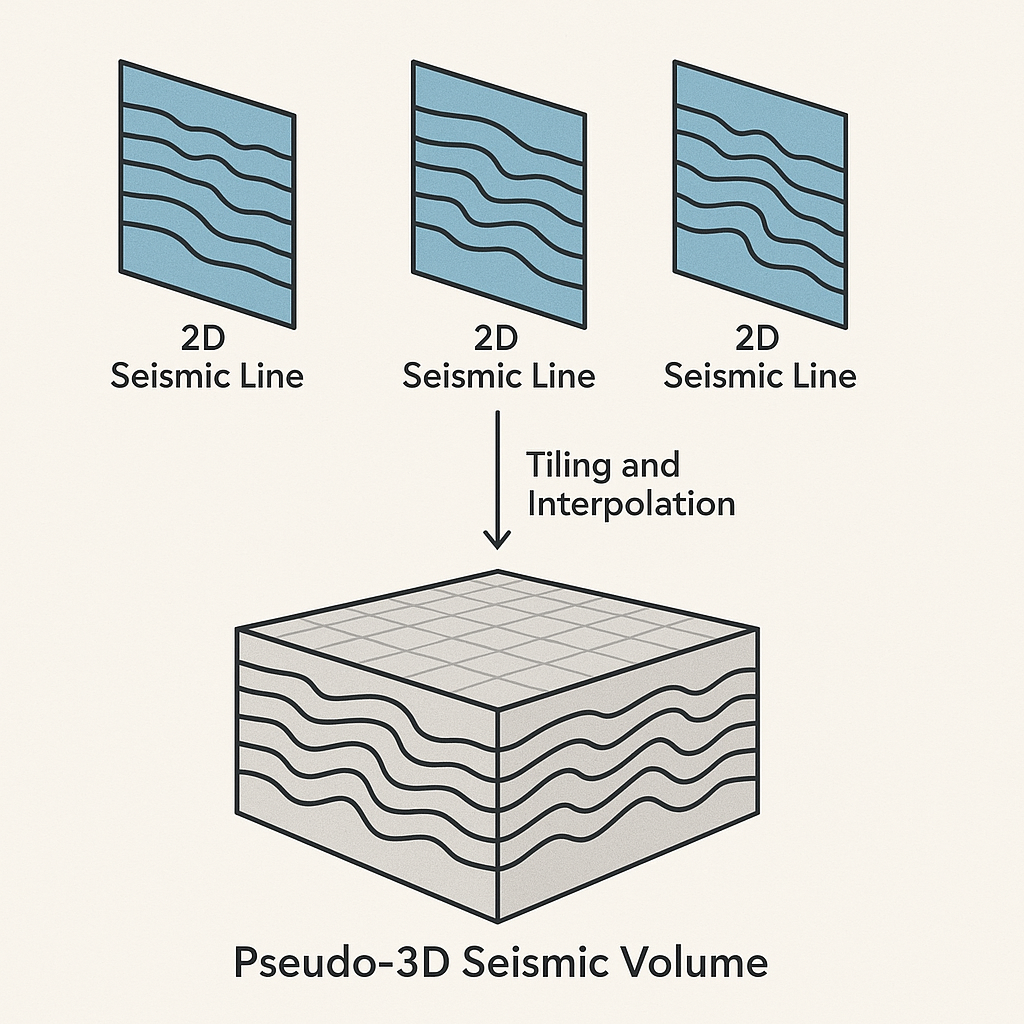
A Pseudo-3D volume is a 3-dimensional seismic dataset created from 2D seismic lines, even though true 3D data was not acquired.
It is called “pseudo” because:
•It simulates a 3D cube
•But it is constructed from 2D profiles, not from dense 3D acquisition
•It is not a true amplitude-preserved 3D dataset
Think of it as stacking and interpolating multiple 2D lines into a 3D grid, giving interpreters a cube-like view where no actual 3D data exists.
Why Create a Pseudo-3D Volume?
You create a pseudo-3D volume when:
✔ You only have several 2D seismic lines (typical in exploration or old data)
✔ You want a 3D-like interpretation environment
✔ You want to visualize horizons and faults across lines
✔ You need to do:
•3D horizon mapping
•Structural modeling
•Fault framework building
•Depth conversion
•Early reservoir evaluation
•Visual QC of 2D alignment
A pseudo-3D cube is NOT used for:
•AVO analysis
•True amplitude studies
•3D inversion
•3D migration
Because it does not have true spatial fold or 3D acquisition geometry.
How a Pseudo-3D Volume Is Created?
1.Import multiple 2D lines into your (g-Platform) software
2.Convert each 2D line into an inline or crossline index
For example:
oLine 1 → Inline 100
oLine 2 → Inline 200
oLine 3 → Inline 300
3.Assign spatial coordinates
Each sample is placed at its true X,Y position.
4.Interpolate between lines (optional)
oLinear
oKriging
oGridding methods - This fills gaps between 2D lines.
5.Write a 3D cube file
Typically SEG-Y 3D or internal volume format.
Where Pseudo-3D Is Commonly Used?
•Early exploration blocks
•Old legacy basins
•Offshore basins with sparse 2D grids
•Areas where 3D acquisition is too expensive
•Government data packages (NDR, NPD etc.)
•Geological modeling of sparse datasets
•
![]()
![]()
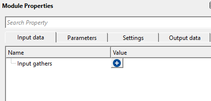
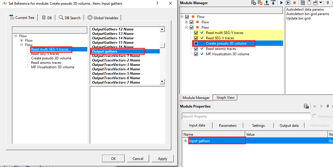
Input gathers - connect/reference to Output gather. For this, we read the input data as multiple 2D lines or combining all 2D lines into a single file. For the former option, we use Read multi SEG-Y traces module. For the later option, we first use concatenate seismic files module to combine all 2D lines into a single file then use Read seismic traces module and change Load data to RAM as YES from NO option.
This is a collection of named input gathers — each entry consists of a Name label and a connected seismic gather. You can connect any number of 2D seismic lines. Each connected line must have its data fully loaded into RAM before this module executes. All input lines are resampled to a common sample interval (set by the DT parameter) before processing. The spatial coordinates (X, Y) stored in the trace headers of each line determine where its traces are placed within the output 3D grid. Ensure that coordinate information in the headers is accurate and in a consistent coordinate reference system.
![]()
![]()
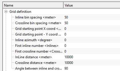
Grid definition - bin grid information is used for creating a 3D grid to accommodate all 2D lines within the 3D bin grid. For the same reason, the user must provide the bin grid information. This can be achieved automatically by clicking "Auto detect bin grid params" option from the action items. Similarly, "Auto detect data params" option for data parameters.
The Grid Definition group specifies the geometry of the output 3D bin grid — that is, the spatial framework into which all input 2D line traces are mapped and interpolated. These parameters define the size, orientation, origin, and numbering of the grid. In most workflows, you do not need to set these values manually: use the Autodetect bin grid params action to compute optimal values automatically from the input data. Manual adjustment is only needed when you want to extend, crop, or rotate the grid relative to the autodetected result.
Inline bin spacing - specify the distance between two adjacent inlines or inline bin distance. Default is 50 m. This value controls how densely the output grid is sampled in the inline direction. A smaller value creates a finer grid but increases the output file size significantly. When using Autodetect bin grid params, this value is set automatically to the average trace spacing measured across all input lines.
Crossline bin spacing - specify the distance between two adjacent crosslines in meters. Default is 50 m. This controls how finely the grid is sampled perpendicular to the inline direction. In a typical pseudo-3D setup this value represents the spacing between the 2D lines themselves, or a fraction of it if you want a denser output grid.
Grid starting point X coord - the easting (X) coordinate of the grid origin — the survey-coordinate position of the first bin corner. This value must be in the same coordinate system as the trace headers of the input seismic data (e.g., UTM meters). Use Autodetect bin grid params to populate this automatically from the data.
Grid starting point - Y coord - the northing (Y) coordinate of the grid origin in the same survey coordinate system as the X coordinate. Together, X and Y define the geographic anchor point from which the entire 3D bin grid is built according to the inline azimuth and bin spacings.
Inline azimuth - the compass bearing (in degrees) of the inline axis direction. An azimuth of 0 means the inline direction runs north; 90 means east. This angle orients the entire bin grid on the map. When lines are not aligned with cardinal directions, Autodetect bin grid params calculates this value from the actual trend of the input lines.
First inline number - the inline index number assigned to the first row of the output 3D grid. Default is 0. This is a labeling parameter: it does not affect the geographic position of the grid, only how inlines are numbered in the output file headers. Set this to match your project's inline numbering convention.
First crossline number - the crossline index number assigned to the first column of the output 3D grid. Default is 0. Like the First inline number, this is a labeling parameter that controls how crosslines are identified in the output headers, without altering the physical grid geometry.
InLine distance - the total spatial extent of the output grid in the inline direction, in meters. Default is 10,000 m. This value, together with Inline bin spacing, determines the total number of inlines in the output cube: approximately InLine distance / Inline bin spacing. Autodetect bin grid params computes this as the bounding box width of all input traces in the inline direction, plus one bin spacing of margin.
Crossline distance - the total spatial extent of the output grid in the crossline direction, in meters. Default is 10,000 m. Together with Crossline bin spacing, this determines the number of crossline traces in the output cube. Set this to cover the full lateral span of your 2D line network in the crossline direction.
Angle between inline and crossline - the angle (in degrees) between the inline and crossline directions. Default is 90 degrees, which produces a standard orthogonal (rectangular) grid. In most surveys inlines and crosslines are perpendicular, so this value should be left at 90. Adjust it only if the input 2D line network is arranged in a skewed or non-orthogonal pattern and you need the output grid to reflect that geometry.
Data length - specify the output record length
The total two-way time length of each output trace, in seconds. Default is 5.0 s. All output traces in the 3D cube will have this length. If the input lines have different record lengths, the module takes the maximum length across all inputs (when using Autodetect data params) to ensure no data is truncated. Set this value to cover your full target depth range. Increasing it beyond the actual data length produces zero-filled samples at the end of each trace.
DT - specify sample interval. By default, 2 ms.
The time sample interval of the output cube in seconds. Default is 0.002 s (2 ms). All input gathers are resampled to this sample interval before interpolation, so the output cube has a uniform sample rate throughout. When multiple input lines have different sample rates, Autodetect data params sets this to the finest (smallest) sample interval found among the inputs to avoid aliasing. Do not set this value coarser than the original data sample rate, as this would discard high-frequency content.
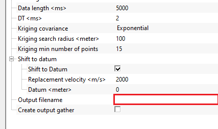
Kriging covariance { Spherical, Gaussian, Exponential } - this is used for interpolation. Krigging uses a covariance model (variogram) to describe how similar two points are depending on the distance between these two points. They are 3 types of covariances
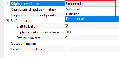
Spherical - this model assumes spatial continuity increases smoothly then becomes constant. Increases from 0 to full correlation and flattens at a distance called range.
Gaussian - Very smooth curve. Correlation drops slowly near the origin but decreases strongly
Exponential - represents noiser data and correlation drops rapidly at short distances however never reaches zero.
The covariance model controls the shape of the spatial weighting function used by the kriging interpolator. Default is Exponential. Choose Spherical when the data shows clear spatial structure up to a certain range and then becomes uncorrelated — this is the most common choice for geological data with a definite range of influence. Choose Gaussian for very smooth, slowly varying data where you want the interpolation to produce the gentlest possible transitions between input traces. Choose Exponential when data variability is high and spatial correlation decays rapidly with distance — the Exponential model gives more weight to the nearest traces and transitions quickly to background. If uncertain, start with Exponential (the default), then compare results with Spherical.
Kriging search radius - the maximum distance from the estimation point from which kriging can search for data points. For example, if the search radius is 1000m, it will consider points within 1000m for interpolation.
Default is 100 m. This is the primary search radius within which the module looks for input traces to use when estimating the value at each output grid node. If at least Kriging min number of points input traces are found within this radius, they are used for interpolation. If fewer traces are found within the search radius, the module automatically expands its search to use the nearest available traces regardless of distance, so interpolation is always attempted at every grid node. Set the search radius to roughly the spacing between your 2D lines: too small a radius will cause the module to frequently fall back to distant traces, while too large a radius will over-smooth the result by mixing data from widely separated lines.
Kriging min number of points - the minimum number of points kriging used for interpolation to estimate the new value.
Default is 15. This is the minimum number of input trace locations that kriging requires to compute a reliable interpolated value. If fewer than this number of traces fall within the Kriging search radius, the module expands its search to the nearest 15 traces (or whatever value is set here). Increasing this number produces smoother results because more surrounding traces contribute to each estimated value, but it may also blend together data from distant 2D lines. Decreasing it allows sparser input configurations to produce output without forced expansion of the search neighborhood, which can preserve local variation but may introduce artifacts in areas with very few nearby traces. A value of 10 to 20 is appropriate for most pseudo-3D workflows.
Shift to datum - it will shift the output volume to final datum
This group controls whether a datum static correction is applied to the input data before kriging interpolation. When input 2D lines are acquired over terrain with varying surface elevations, each trace may have a different time reference (floating datum). Shifting all traces to a common flat datum ensures that reflections at the same depth arrive at the same two-way time across all traces, which is essential for coherent 3D interpolation. If your input data has already been reduced to a floating datum or has negligible topographic relief, you can leave this correction disabled.
Shift to Datum - enable or disable the datum static correction. Default is enabled (true). When enabled, each input trace is shifted in time by the amount needed to bring its reference elevation to the flat Datum level, using the Replacement velocity for the travel-time calculation. This correction is applied before kriging so that the interpolation operates on datum-consistent data. Disable this option only if all input lines already share the same datum elevation.
Replacement velocity - the velocity (in m/s) used to convert elevation differences into time shifts when applying the datum correction. Default is 2000 m/s. This value represents the assumed propagation speed in the near-surface weathering layer, between the surface and the datum plane. Use the average near-surface velocity of your survey area. A typical value for consolidated sediments is 1800–2500 m/s; use a lower value for soft soils or weathered rock. This parameter has no effect when Shift to Datum is disabled.
Datum - the target flat datum elevation (in meters) to which all input traces are shifted. Default is 0 m (sea level). Set this to the elevation of the flat reference plane for your processing project — typically the project datum defined during geometry assignment. When Autodetect data params is used, this value is set automatically to the maximum surface elevation found across all input traces, which is a conservative choice that avoids upward shifting any trace beyond the top of the record.
Output filename - provide the final output pseudo 3D volume name.
The file path and name for the output pseudo-3D volume, saved in g-Platform's native binary format (.gsd). This file is written during execution and can subsequently be loaded as a 3D seismic volume for visualization (inline/crossline/time-slice views), horizon picking, and other interpretation workflows. Ensure the destination folder has sufficient disk space — output volume size is approximately: (number of inlines) x (number of crosslines) x (Data length / DT) x 4 bytes.
Create output gather - this option allows the user to create output gather.
Default is disabled (false). When enabled, the completed 3D cube is also exposed as an in-memory output gather item (connected to the Output gather data item), in addition to being written to the output file. This allows you to chain further processing steps — for example, viewing the result in a Vista display window or feeding it into a subsequent module — without loading the file back from disk. Note that for large surveys, keeping the full cube in memory can require significant RAM.
![]()
![]()
Skip - By default, FALSE(Unchecked). This option helps to bypass the module from the workflow.
![]()
![]()
Output gather - generates output pseudo 3d volume
The in-memory representation of the completed pseudo-3D volume, available as a data item for downstream modules. This output is only populated when Create output gather is enabled. When populated, the output gather contains all traces of the 3D cube organized by bin, with inline and crossline indices, spatial coordinates, and datum elevation written into each trace header. You can connect this output to a Vista 3D display node, a stacking module, or any other module that accepts a seismic gather as input.
There is no information available to this module so the user can ignore it.
![]()
![]()
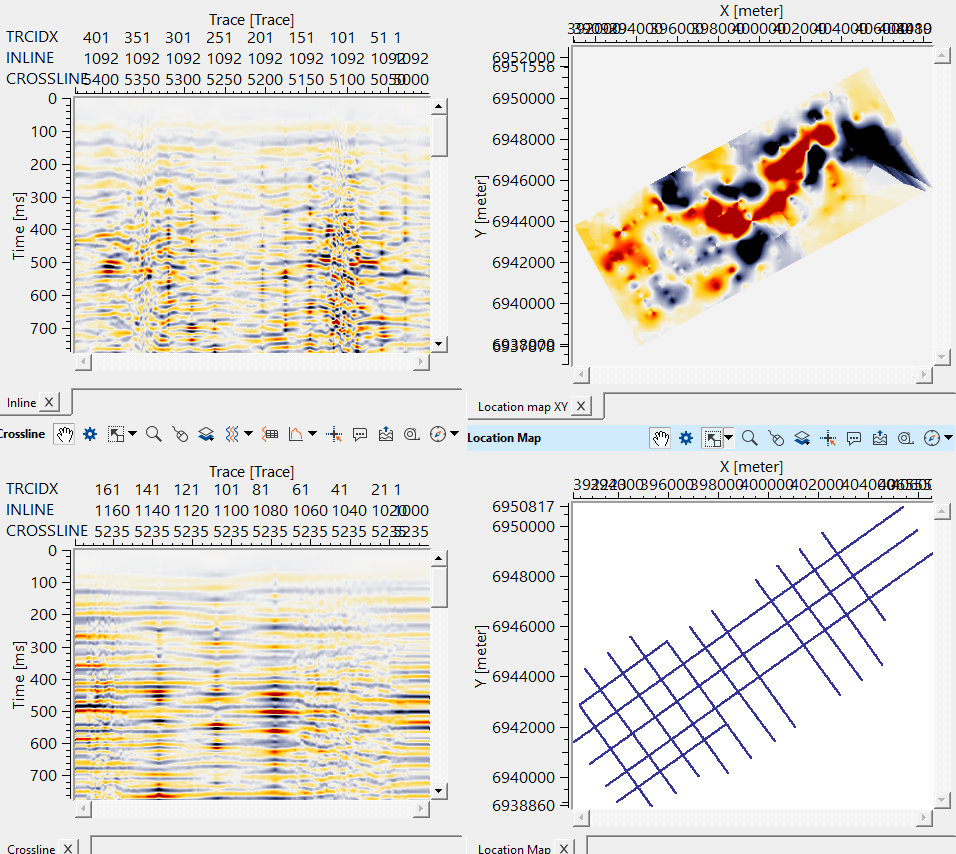
In this example workflow, we are reading multiple 2D lines by using "Read multi SEG-Y traces" module. The output dataitem will be connected to Create pseudo 3D volume.
![]() Read multi SEG-Y traces must have load data to RAM as YES
Read multi SEG-Y traces must have load data to RAM as YES
For Parameters, we can automatically detect the Grid definition and Data length, DT from the action items menu.
Setup all the parameter and give an output file name against the Output file name parameter and execute the module.
Launch Vista items. It will generate, Inline, Crossline, Location map etc.
Test Kriging search radius and minimum number of points. These are the key parameters for the better interpolation.
![]()
![]()
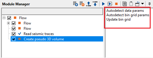
Autodetect data params - this option automatically detects the data parameters of the input files.
Scans all connected input gathers and automatically sets Data length, DT, and Datum to values derived from the input data: the maximum record length, the finest sample interval, and the highest surface elevation across all input traces, respectively. Run this action after connecting all input gathers and before executing the module, so that the output cube covers all input data without truncation.
Autodetect bin grid params - this options detects the bin grid parameters from the input files.
Analyzes the spatial positions of all input traces and automatically computes the optimal Grid Definition parameters: the grid origin (X, Y coordinates), inline azimuth, inline and crossline bin spacing (set to the average trace spacing), and the inline and crossline distances needed to contain all input data. It also refreshes the Created bin grid visualization so you can inspect the grid layout on the map. Run this action before executing the module to avoid having to set grid parameters manually. After running it, you can still fine-tune individual parameters (for example, to extend the grid boundary or adjust numbering).
Update bin grid - in case the user provides bin grid parameters, it will update the bin grid.
Recomputes and redraws the Created bin grid visualization from the current Grid Definition parameter values without changing any parameter values. Use this action after manually editing any grid parameter (for example, after adjusting the Inline bin spacing or Inline azimuth) to immediately see how the updated grid covers the input lines. This is a visual QC tool: it does not trigger module execution.
![]()
![]()
YouTube video lesson, click here to open [VIDEO IN PROCESS...]
![]()
![]()
Yilmaz. O., 1987, Seismic data processing: Society of Exploration Geophysicist
 * * * If you have any questions, please send an e-mail to: support@geomage.com * * *
![]()