Source and receiver ghost-waves attenuation
The Deghost module attenuates ghost reflections from marine seismic data by applying an iterative least-squares inversion in the frequency-wavenumber (F-K) domain. Ghost waves are upward-travelling reflections that bounce off the sea surface before being recorded; they create notches in the frequency spectrum and degrade vertical resolution. This module removes the ghost response from both source and receiver sides simultaneously, restoring broad-band frequency content and sharpening reflectors. It is designed for pre-stack common-shot or common-receiver gathers, and supports an optional stack-mode path for post-stack or near-stack data.
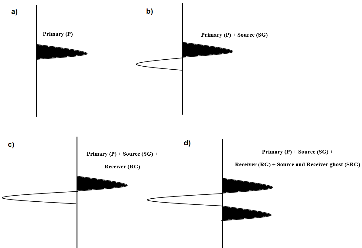
Figure 1. Ghost waves generation scheme.
Ghost notch frequencies are determined by the depth of the source or receiver below the sea surface. The notch frequencies follow the formula:
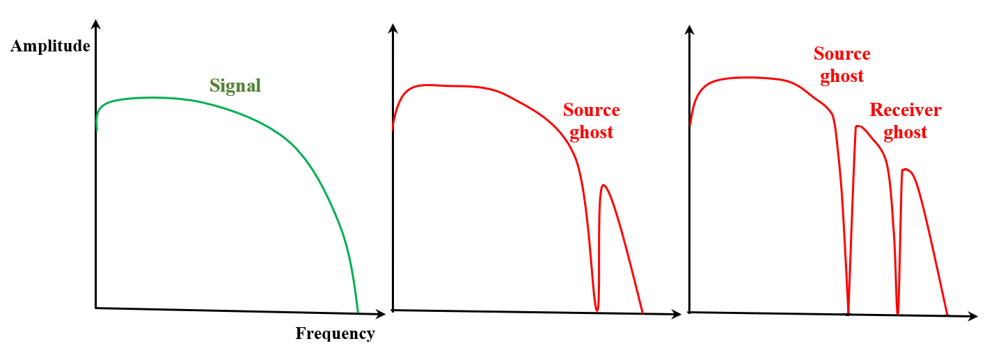
where V is the water velocity (m/s) and Depth is the towing depth of the source or receiver (m). For example, a streamer towed at 6 m depth with a water velocity of 1500 m/s will produce notches at 0 Hz, 125 Hz, 250 Hz, etc. Deghosting inverts this effect to restore the full frequency spectrum, as illustrated below.
For pre-stack gathers, the module builds a 2D F-K ghost operator that models the phase shift introduced by the free-surface reflection at the source or receiver towing depth. It then solves for the deghosted wavefield using one of the iterative least-squares solvers (LSQR or FISTA). Amplitude balancing via AGC is optionally applied before inversion and reversed afterwards, to stabilize the numerical solution when trace amplitudes vary strongly with offset. A direct-wave mute mask — computed from the water velocity and source-receiver geometry — prevents the solver from modifying the first-arrival energy above the expected water-wave travel time.
Input DataItem
Connect a seismic gather in the time domain. The input must be a pre-stack common-shot or common-receiver gather sorted by offset, or a post-stack gather when running in stack-solve mode. The module reads source and receiver towing depths from the trace headers automatically when the Use depth from trace headers option is enabled. The gather type (common shot vs. common receiver) is detected automatically from the header geometry.
V0 - Water velocity (m/s).
The acoustic velocity of seawater, in m/s. Default: 1560 m/s. This value is used in two places: (1) to compute the F-K ghost operator (the phase shift depends on water velocity), and (2) to define the direct-wave mute curve that protects the first-arrival energy from being modified. A typical range for marine surveys is 1480–1530 m/s for temperate waters; values up to 1560 m/s may apply in warmer seas. Use the actual measured or estimated water velocity for your survey area — an incorrect value will shift ghost notch positions and degrade the deghosting quality.
T0 - Start time for processing.
The two-way travel time of the direct wave at zero offset, in seconds. Default: 0.035 s (35 ms). Together with V0 and the trace offset, this value defines a hyperbolic mute curve that blanks all samples above the expected direct-wave arrival. Samples earlier than this muted zone are set to zero both before and after deghosting, ensuring that the near-surface direct-wave energy is not altered by the inversion. Set T0 to approximately 2 * source_depth / V0 to correctly position the mute at zero offset. If the mute is too early (T0 too small), some direct-wave energy may survive and contaminate the deghosted output. If it is too late, shallow reflector energy near the water bottom may be incorrectly zeroed.
Mute above v0
When enabled (default: on), the module applies a hyperbolic mute mask to zero all trace samples above the direct-wave travel-time curve before running the deghosting inversion, then re-zeros those same samples in the output gather. The mute curve is computed per trace from the offset, V0, and T0. Disable this option only if you have already applied a direct-wave mute to your data upstream, or if your gather does not contain a direct wave (for example, a receiver gather where the direct wave has been removed).
Use depth from trace headers
When enabled (default: on), the towing depth of the source and receiver is read directly from the trace headers (the holeDepth field of the source and receiver records). This is the recommended setting when the geometry has been correctly populated from the field acquisition system. When disabled, the Source water depth and Receiver water depth parameters below become active and must be set manually to constant values.
Source water depth
The towing depth of the seismic source below the sea surface, in meters. Default: 0 m. This parameter is active only when Use depth from trace headers is disabled. For common-receiver gathers, this depth is used to model and remove the source ghost. Typical airgun array depths range from 4 to 10 m. A depth of zero will cause an error — the deghosting operator cannot be constructed without a non-zero depth value.
Receiver water depth
The towing depth of the hydrophone streamer below the sea surface, in meters. Default: 0 m. This parameter is active only when Use depth from trace headers is disabled. For common-shot gathers, this depth is used to model and remove the receiver ghost. Typical streamer towing depths range from 4 to 15 m depending on the target frequency bandwidth. A depth of zero will cause an error.
Solver parameters
This group controls the iterative inversion algorithm used to solve for the deghosted wavefield. The deghosting problem is formulated as a least-squares minimisation where the forward operator models how the ghost reflection contaminates the recorded data. Three solver algorithms are available, each suited to different data characteristics.
Solver type
Selects the algorithm used to solve the deghosting inversion. Default: LSQR. Three options are available:
LSQR — the standard Least Squares QR algorithm. This is the recommended choice for most datasets. It converges reliably and is computationally efficient. The Damping coefficient and Tolerance parameters control regularisation and early stopping.
LSQR advance — an extended LSQR variant that applies an adaptive subtraction step using the ghost-shifted trace as a model. This may provide better ghost cancellation on data with non-stationary amplitude behaviour across the gather, at the cost of longer computation time.
FISTA — the Fast Iterative Shrinkage-Thresholding Algorithm, a proximal gradient method with L1 sparsity regularisation. This solver can suppress residual noise more aggressively than LSQR by promoting a sparse solution in the transform domain. Use when the data has a high noise level and LSQR leaves visible artefacts, but expect longer computation times.
Number of iterations
The maximum number of iterations the solver will perform before stopping. Default: 1000 (minimum: 1). The solver may also stop early if the residual drops below the Tolerance threshold. For most well-conditioned datasets, convergence is achieved well below 1000 iterations; reducing this value (e.g. to 100–200) can significantly speed up processing at the cost of a slightly less accurate solution. Increase if the output shows residual ghost energy and the solver has not yet converged (check by running with a higher iteration count and comparing outputs).
Damping coefficient
Tikhonov regularisation factor applied to the LSQR inversion. Default: 0 (range: 0–1). A value of 0 means no damping; the solver minimises the data misfit alone. Increasing damping adds a penalty on the solution energy, which stabilises the inversion when the data is noisy or the ghost operator is poorly conditioned at low signal-to-noise frequencies. Start with small values such as 0.01–0.05 and increase if the output shows noise amplification or ringing near the ghost notch frequencies. Excessive damping will suppress the deghosting effect.
Tolerance
The convergence tolerance used as an early stopping criterion for the solver. Default: 1e-4 (minimum: 1e-8). The solver stops when the relative residual norm falls below this value. For most surveys, the default of 1e-4 provides sufficient accuracy. Tighten the tolerance (e.g. to 1e-6) if residual ghost energy is visible in the output and the iteration count has not yet been reached. Loosen it (e.g. to 1e-3) to speed up processing when a slightly approximate solution is acceptable.
Advanced parameters
This group contains options that control the data conditioning, padding, and alternative processing modes. These settings can be left at their defaults in most situations and adjusted only when specific problems are observed in the output.
Solve as stack
When enabled (default: off), treats each trace in the gather independently as a 1D single-trace deghosting problem rather than solving the full 2D F-K gather inversion. In this mode the ghost is modelled as a simple time-shifted and sign-inverted copy of the primary, and the least-squares solution finds the best deghosted trace for each record individually. This mode is suitable for post-stack data or for gathers where the offset structure is not well sampled. When enabled, the Stack solve side option becomes visible.
Stack solve side
Visible only when Solve as stack is enabled. Default: S side. Selects which ghost (source ghost, receiver ghost, or both) is removed in single-trace stack mode. S side removes the source ghost; R side removes the receiver ghost; S-R side applies both operations sequentially to each trace. Each removal step uses the corresponding depth read from the trace header or set manually in the depth parameters above.
Split positive and negative offsets
Visible only when Solve as stack is disabled (pre-stack mode). Default: off. When enabled, the gather is split into two sub-gathers containing negative-offset and positive-offset traces respectively, each processed by a separate F-K inversion, and then recombined. Enable this option when the gather contains both positive and negative offsets from a split-spread acquisition geometry, or when asymmetric streamer configurations cause the negative-offset and positive-offset traces to have different wavenumber sampling characteristics. The two sub-gathers are merged back after deghosting with amplitude weighting proportional to the maximum absolute offset of each sub-gather.
Padding size
Visible only in pre-stack mode. The number of zero traces added to the edges of the gather before F-K transformation, to reduce wraparound artefacts from the spatial Fourier transform. Default: 0 traces. Use a non-zero value (typically 10–30 traces) when the first or last traces of the gather have strong energy that would alias across the F-K boundaries. Padding increases computation time proportionally to the number of added traces.
Taper window
Visible only in pre-stack mode. The half-width in traces of a cosine taper applied to both edges of the gather before F-K transformation. Default: 0 traces (no tapering). Setting a taper window (e.g. 5–15 traces) smoothly reduces the edge amplitudes to zero before the F-K transform, which reduces spectral leakage and edge-related artefacts in the deghosted output. This is especially useful when the gather traces have strong amplitudes at near or far offsets. The taper is applied asymmetrically — it affects the forward transform but is compensated via the adjoint operator during inversion.
Use AGC
When enabled (default: on), an Automatic Gain Control is applied to the input gather before the inversion, and the inverse gain function is applied to restore the original amplitude envelope after deghosting. This balances the trace amplitudes so that far-offset traces with weaker signal do not become under-represented in the least-squares solution. The AGC is purely a numerical conditioning step — it does not affect the relative amplitudes of the final output because the gain is exactly reversed afterwards. Disable only if your data already has balanced amplitudes, or if preserving the amplitude relationships within the inversion is critical for research purposes.
AGC window
Visible only when Use AGC is enabled. The length of the sliding window used to compute the AGC envelope, in seconds. Default: 0.5 s. A shorter window provides tighter amplitude balancing within each trace but may over-normalise weak signal zones. A longer window applies a smoother gain curve that better preserves large-scale amplitude trends. For typical marine data with a record length of 4–8 s, a value of 0.3–1.0 s is appropriate.
Bad data values option
There are 3 options for corrupted (NaN) samples in trace:
1. Fill bad values with zeros before solving - the solver sees zeros in place of bad samples. This avoids NaN propagation and is suitable when the fraction of bad samples is small.
2. Restore bad values after solving - bad samples are reinserted from the original trace into the deghosted output, so the output retains the same bad-sample mask as the input.
3. Skip traces containing bad values - any trace that contains at least one NaN sample is passed through without modification. Use this option when bad traces should be excluded from the deghosting process entirely.
The interactive seismic display shows a Direct waves cutter overlay (a bold line in the gather view) that represents the computed mute curve for the current V0 and T0 settings. Use this visual guide to verify that the mute correctly follows the direct-wave arrival before running the full processing job.
Output DataItem
The deghosted seismic gather in the time domain. The output has the same number of traces, samples, and sample interval as the input. Ghost reflections are attenuated and the associated frequency notches are filled, resulting in a broader bandwidth wavelet and improved vertical resolution. The direct-wave mute zone (above the V0/T0 hyperbola) is zeroed in the output regardless of the solver result. All trace headers are preserved unchanged from the input.
Figure 2. Deghosting workflow in g-Platform.
An example of the workflow for deghosting:
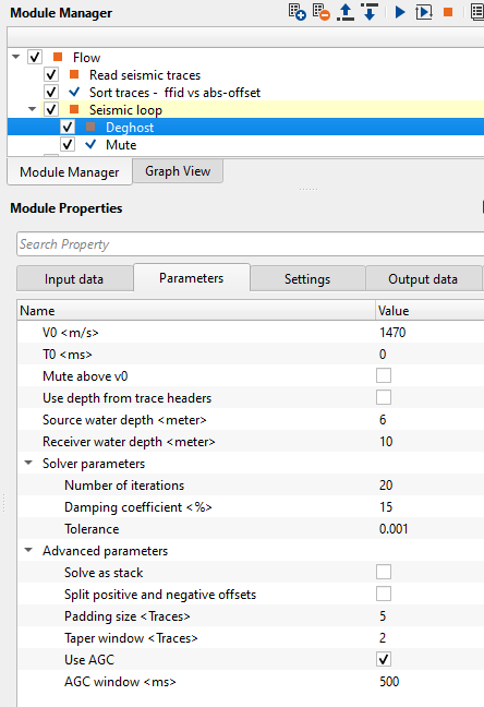
Figure 3. Deghosting module parameter panel.
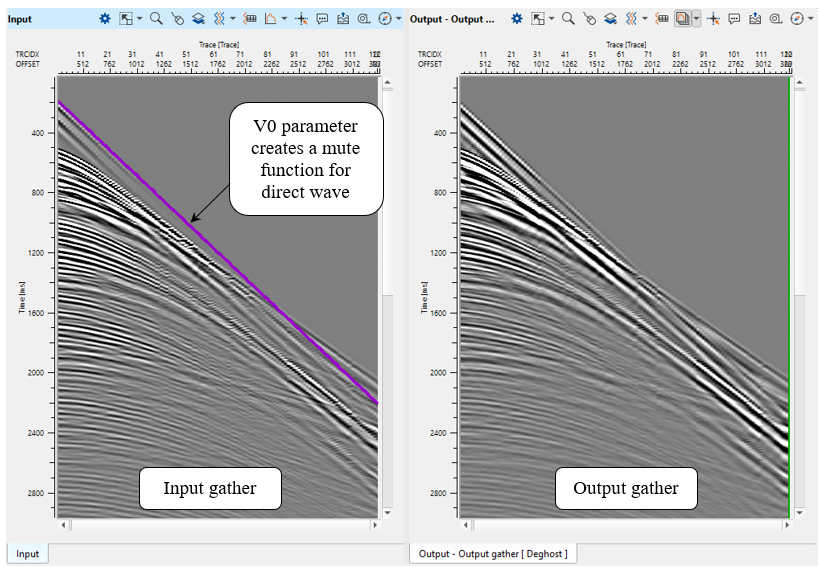
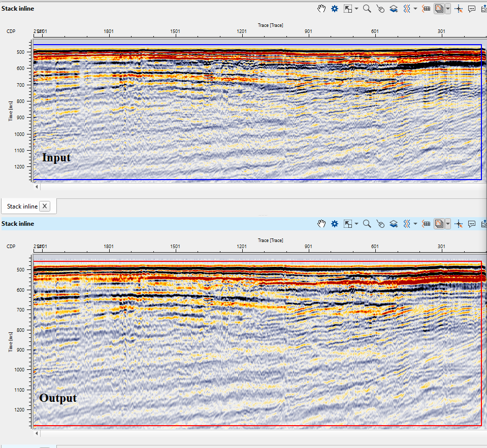
Figure 5. Source gather before (left) and after (right) deghosting procedure.

Figure 6. Amplitude frequency spectrum before (red) and after (green) deghosting procedure.
Spectral analysis after the Deghost. We can clearly see that the low frequency is boosted up and the notch is removed after the deghosting.
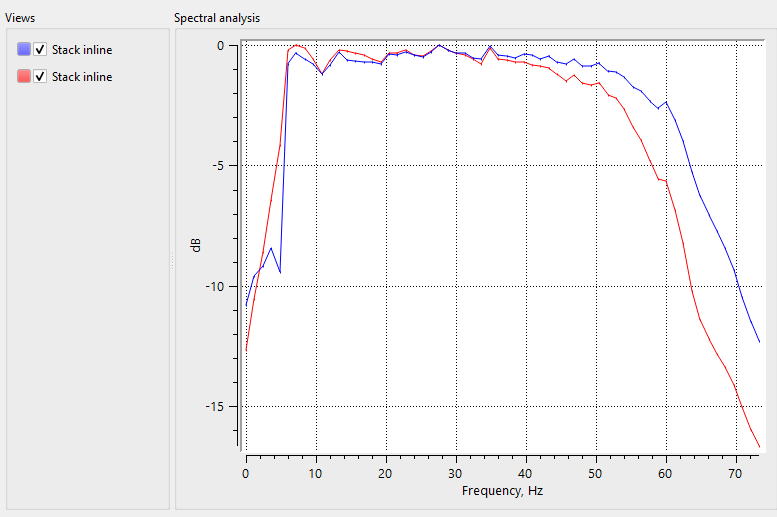
Figure 4. Comparison of gather displays and F-K spectra before and after deghosting.
This modules doesn't have any action items so the user can ignore it.
References:
![]()
![]()
Yilmaz. O., 1987, Seismic data processing: Society of Exploration Geophysicist