Interpolating the trace headers information in matrix format
Description
The Create Interpolation Matrix module builds a regular 2D spatial grid of interpolated values from scattered point data. The input data can originate from seismic trace headers (for example, source or receiver elevations, static shifts, or any per-trace attribute), from an external ASCII/table file, or from a point vector item. The module places each input point on a defined rectangular grid and then fills every grid node with an interpolated value using one of three spatial interpolation methods: ABOS (approximation based on smoothing), Triangulation, or Kriging.
Use this module when you need to convert irregularly distributed geophysical measurements — such as borehole-derived static corrections, surveyed elevations, or modelled velocity values — into a continuous surface that can subsequently be applied across the full survey area. The resulting interpolation matrix can be consumed by downstream modules that require a spatially regular grid of values.
Parameters
The module parameters are organised into four groups: the data source selector, the group-specific source settings (Table properties or Trace headers properties), the Interpolation properties, and the Grid definition. Only the parameter group that corresponds to the selected input source is active at any time.
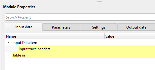
Input DataItem
The module accepts up to three optional input data connections, depending on the selected data source:
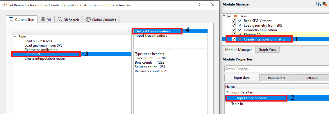
Trace vector (geometry input): Required when Input from is set to Trace headers. This is the seismic geometry data item that carries all trace header fields such as source X/Y coordinates, receiver X/Y coordinates, CMP coordinates, fold, offset, and any custom attributes attached during geometry assignment.
Table in: Required when Input from is set to Table. Connect an ASCII table item that contains at minimum three named columns: the X coordinate column, the Y coordinate column, and the value column. The column names are mapped using the Table properties parameters below.
Input points vector: Required when Input from is set to Point vector. Connect a point vector item in which each point carries an X coordinate, a Y coordinate, and a scalar value (Z component) to be interpolated.
Input from
Selects the data source from which the scattered spatial points and their associated values are read. Choose one of:
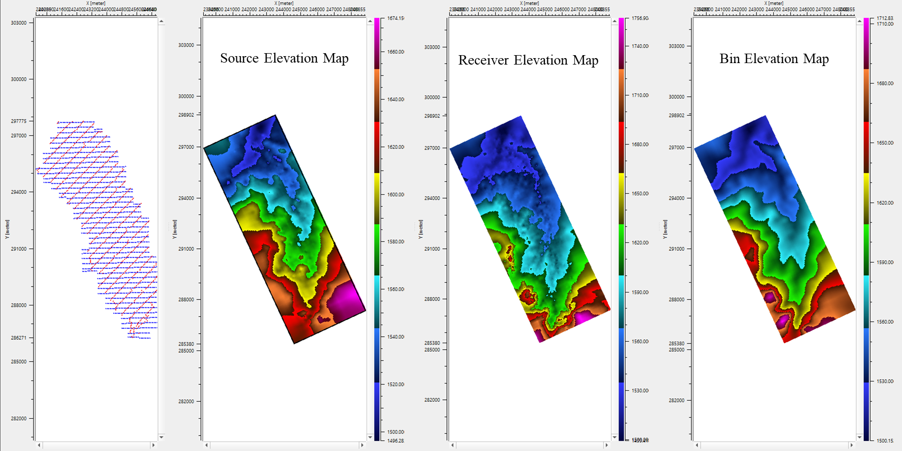
Trace headers (default) — the module reads X/Y positions and the attribute value to be interpolated directly from the seismic geometry trace headers. Use this option to produce a spatial map of any per-trace attribute, such as source or receiver elevation, residual static, offset, or a custom computed header field.
Table — the module reads points from a connected table data item. The columns for X, Y, and the scalar value are specified in the Table properties group. Use this option when the data comes from an external source such as a well database, a survey spreadsheet, or a previously exported attribute file.
Point vector — the module reads points from a connected point vector item, where the Z component of each point is the value to be interpolated. Use this option when the point data has already been assembled in memory by a preceding module in the processing flow.
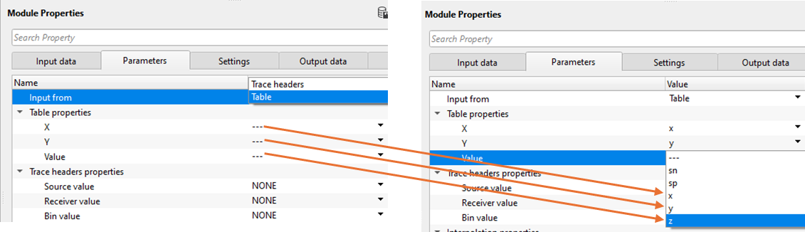
Table properties
This group is active only when Input from is set to Table. Map the three required columns from the connected table to their geophysical roles.
X: Select the table column that contains the easting (X) coordinate of each data point, in the same coordinate system as the survey grid. Default column name: X.
Y: Select the table column that contains the northing (Y) coordinate of each data point. Default column name: Y.
Value: Select the table column that contains the scalar value to be interpolated at each (X, Y) location — for example, elevation, static correction in milliseconds, or a velocity value. Default column name: Value.
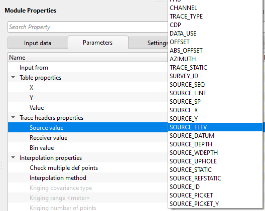
Trace headers properties
This group is active only when Input from is set to Trace headers. At least one of the three header selectors must be set to a value other than NONE.
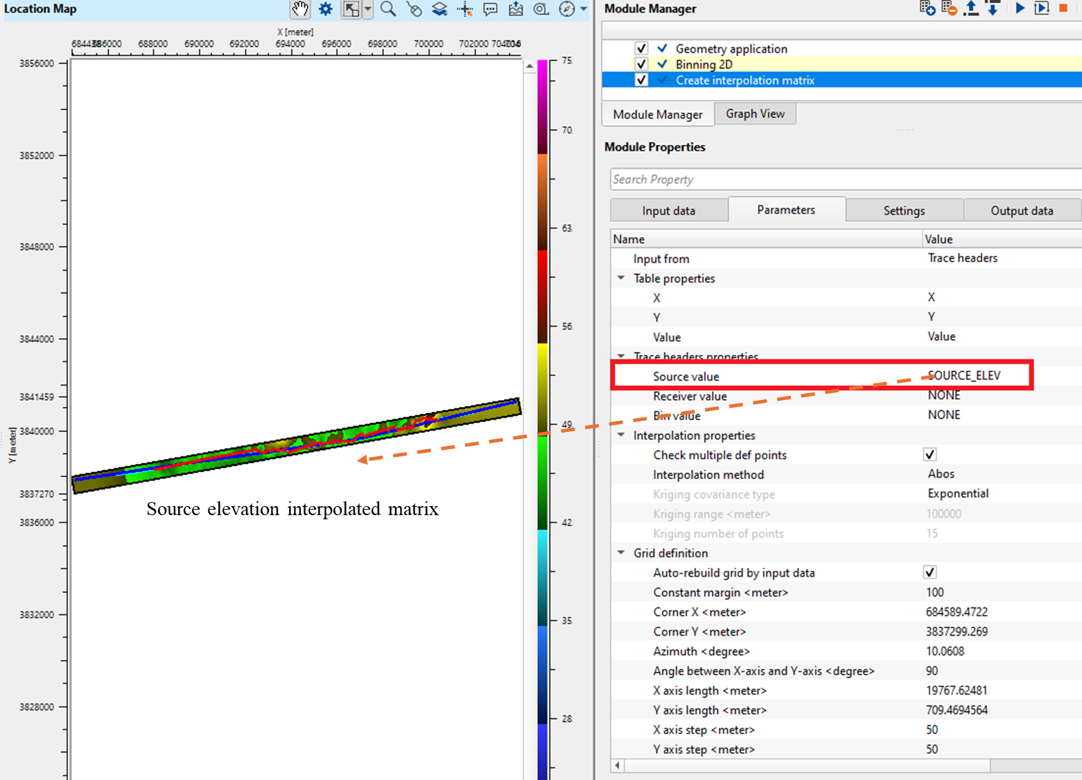
Source value: Select the trace header field whose value will be plotted at each source location and included in the interpolation. Set to NONE to exclude source positions from the interpolation. Typical choices include source elevation, source static correction, or any custom source header. Default: NONE.
Receiver value: Select the trace header field whose value will be plotted at each receiver location and included in the interpolation. Typical choices include receiver elevation, receiver static correction, or any custom receiver header. Set to NONE to exclude receiver positions. Default: NONE.
Bin value: Select the trace header field whose value will be plotted at each CMP/bin centre location and included in the interpolation. Typical choices include fold, offset, or CMP-averaged attributes. Set to NONE to exclude bin-centre positions. Default: NONE.
Interpolation properties
Controls how the scattered input values are interpolated onto the regular output grid.
Check multiple definition points: When enabled (default: on), the module verifies that no two input points share the same spatial coordinates but carry different values. If such conflicting points are found, execution stops and an error is reported. Disable this check only when you intentionally have overlapping points and wish to average or ignore duplicates. Keeping this check enabled is strongly recommended during initial data quality control.
Interpolation method: Selects the algorithm used to fill grid nodes from the scattered input points. Three options are available:
Abos (default) — Approximation Based On Smoothing. This method fits a smooth surface to the input points using a minimum-curvature approach. It produces naturally smooth results and handles irregularly distributed data well. This is the recommended choice for most geophysical attributes such as elevation grids or static correction maps.
Triangulation — Delaunay triangulation with barycentric weight interpolation. Grid nodes inside the convex hull of the input points are interpolated exactly between the triangulated vertices; nodes outside the hull receive an extrapolated value. This method is fast and honours the input data values exactly, making it suitable for attribute grids where the data is dense and already well-distributed.
Kriging — Geostatistical interpolation that uses a variogram model (covariance function) to optimally weight neighbouring data points. Kriging is the most rigorous method and is well-suited for spatially correlated geophysical quantities such as reservoir thickness or formation depth, but it requires more computation time and the user must specify a covariance model and range. When Kriging is selected, three additional parameters become active.
Kriging covariance type: (Kriging only) Selects the mathematical model that describes how spatial correlation decays with distance. Options are Exponential (default), Spherical, and Gaussian. The Exponential model provides a gradually tapering correlation and is the most robust general choice. The Spherical model reaches zero correlation at exactly the specified range, making it appropriate when there is a known limit of spatial influence. The Gaussian model produces very smooth interpolated surfaces and is suitable when the attribute is expected to vary slowly and continuously.
Kriging range (m): (Kriging only) The spatial correlation length, in metres, beyond which two points are treated as statistically independent. Points closer together than this distance have a strong influence on each other; points further apart contribute little. Set this value to approximately the characteristic spacing of your data or to the geologically meaningful correlation length of the attribute being interpolated. Default: 100,000 m. Reduce this value if you want the interpolation to be more local; increase it to produce a smoother, more regionally influenced surface.
Kriging number of points: (Kriging only) The maximum number of nearest neighbouring data points used to estimate the value at each grid node. Using more points increases accuracy but significantly increases computation time. Using fewer points makes computation faster but may reduce the quality of the interpolation in areas of sparse data. Default: 15. Values in the range of 10 to 30 are typical for seismic attribute grids.
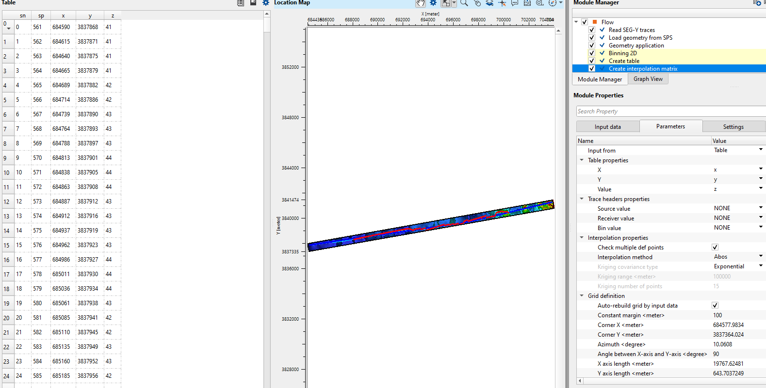
Grid definition -
Defines the geometry of the regular output matrix: its spatial extent, orientation, and sampling interval. All distance parameters are in metres.
Auto-rebuild grid by input data: When enabled (default: on), the module automatically calculates the grid bounding box from the spatial extent of the input data points. The corner coordinates, axis lengths, and azimuth are then populated automatically and the manual grid definition parameters below are ignored. Disable this option when you need to produce a matrix with a precisely controlled spatial extent, for example to match an existing seismic survey grid or a previously defined processing grid.
Constant margin (m): An additional border, in metres, added around the data extent when the grid is built automatically. A positive value expands the grid beyond the outermost data points, ensuring that edge effects in the interpolation do not affect the usable area. Default: 100 m. Increase this value for Kriging to reduce boundary artefacts.
Corner X (m): The easting coordinate of the grid origin corner, in the project coordinate system. Used only when Auto-rebuild grid by input data is disabled. Default: 0.
Corner Y (m): The northing coordinate of the grid origin corner. Used only when Auto-rebuild grid by input data is disabled. Default: 0.
Azimuth (degrees): The compass bearing of the grid X axis, measured clockwise from geographic north. Set this to match the dominant line direction of your seismic survey so that the grid rows and columns align with the inline/crossline orientation. Default: 90 degrees (grid X axis pointing east).
Angle between X-axis and Y-axis (degrees): The angle between the grid X axis and the grid Y axis. For a standard orthogonal grid this should be 90 degrees (default). Changing this value creates a skewed (non-orthogonal) grid, which can be useful for surveys acquired along crooked lines or with non-rectangular geometries.
X axis length (m): The total extent of the grid along the X axis, in metres. Used only when Auto-rebuild grid by input data is disabled. Default: 10,000 m.
Y axis length (m): The total extent of the grid along the Y axis, in metres. Default: 10,000 m.
X axis step (m): The spacing between adjacent grid nodes along the X axis, in metres. A smaller step produces a finer, higher-resolution output matrix but increases computation time and memory usage. Set this to approximately the typical source or receiver spacing along the X direction. Default: 50 m.
Y axis step (m): The spacing between adjacent grid nodes along the Y axis, in metres. Set to match the typical source or receiver line spacing. Default: 50 m.
Auto-connection - By default, TRUE(Checked).
When Auto-connection is enabled, g-Platform automatically links the output Interpolation Matrix item to compatible downstream modules in the processing flow. This saves manual wiring and is the recommended setting in most workflows. Disable this option only if you need precise manual control over which downstream module receives the matrix output.
Output DataItem -
Interpolation matrix: The primary output of this module. It is a regular 2D grid (matrix) in which every node holds the interpolated scalar value at that spatial location. The grid geometry (cell size, orientation, and extent) is determined by the Grid definition parameters. This matrix item can be connected to downstream modules — for example, to apply a spatially variable static correction, to create a velocity model surface, or to display a colour-coded attribute map in the 2D map view.
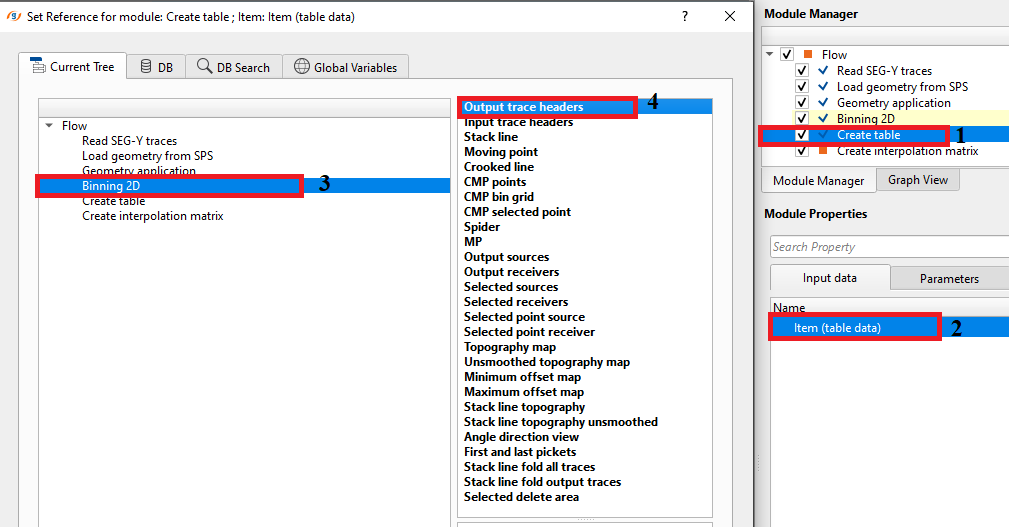
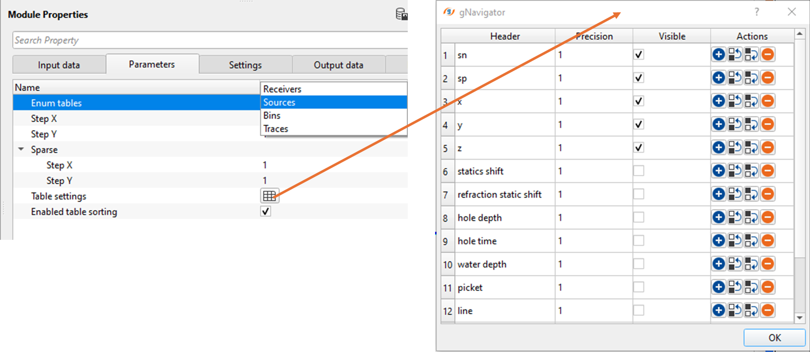
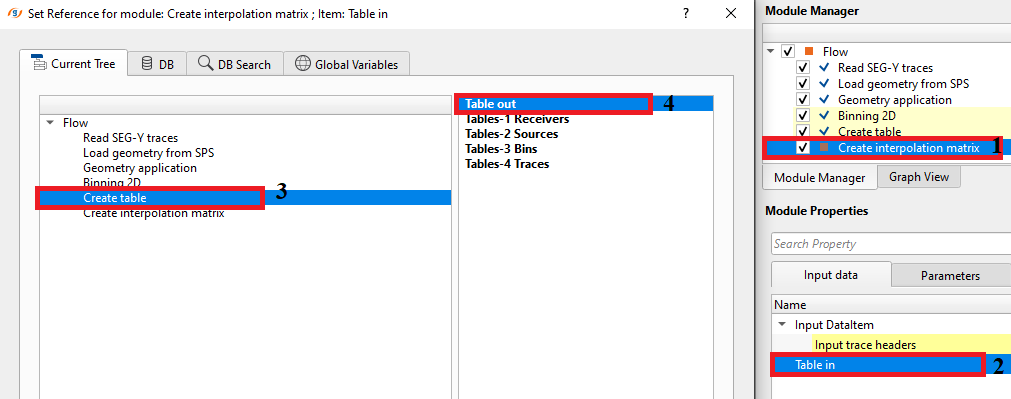
In case of Table, how do we create the interpolation from the Table?
There are no actions available for this module so the user can ignore it.
![]()
![]()
Yilmaz. O., 1987, Seismic data processing: Society of Exploration Geophysicist