Random noise attenuation (Prestack / Poststack)
![]()
![]()
Cadzow De-Noise Filter is based on rank reduction of matrix on frequency slices to attenuate the random noise. This can be done in pre and/or post stack data. Even though the parameters are similar to RNA (Random Noise Attenuation) module, the working principle is slight different as far as the Eigen values are concerned. In this case, these Eigen vectors are applied on multiple dimensions (3 or more) unlike the two dimensions in RNA. The other advantage of Cadzow De-Noise Filter is that it can work on flat or dipping events. It preserves the dips of steeply dipping events while attenuating the random noise.
![]()
![]()
No actions
![]()
![]()
Prestack or post stack seismic data, any sorting.
![]()
![]()
Horizontal sliding window <Traces>
Number of traces for creating spatial sliding window.
This parameter controls the lateral extent of the analysis window. The window slides across the gather trace by trace, and all traces within the window are used jointly to construct the Hankel matrix on which rank reduction is performed. The default value is 40 traces. A wider window captures more spatial coherence and typically produces stronger noise attenuation, but increases computation time. Use a narrower window when the geology contains rapid lateral variations or when the data are sparse. Ensure this value is larger than the Number of Eigen Values to avoid an underdetermined system.
Time interval in milliseconds for creating spatial sliding window. Usually starts from 50 ms, there may be artifacts on the output image in case of too small window
The vertical (temporal) extent of the sliding analysis window, specified in seconds. The default value is 0.05 s (50 ms). The window slides along the time axis in steps; at each position, the samples within this time range are used to build the frequency-domain matrix. Values below approximately 50 ms often cause visible banding artifacts in the output because the frequency resolution becomes insufficient to separate signal from noise. Larger windows provide better frequency resolution and smoother results, but they assume that the data are stationary over a longer time interval. Increase this value for low-frequency content or strongly varying wavelet character.
A cosine taper applied to the edges of the time analysis window before processing, specified in seconds. The default value is 0.05 s (50 ms). Tapering reduces spectral leakage caused by abrupt edge truncation of the windowed data segment, which can introduce artificial frequency components that impair the rank-reduction step. A taper length of 0 disables tapering entirely. Increasing the taper length smooths window-edge discontinuities more aggressively, which can further reduce edge artifacts, but effectively shortens the analysis bandwidth of the time window. This value should be smaller than the Time window parameter.
Start frequency for processing.
The lowest frequency, in Hz, to include in the noise attenuation process. The default value is 0 Hz (no lower cutoff). Rank reduction is applied independently to each frequency slice between Min frequency and Max frequency. Frequencies below this threshold are passed through unmodified. Raise this value to protect very low-frequency content (for example, long-period ground roll remnants that should be kept) from being affected by the filter.
End frequency for processing.
The highest frequency, in Hz, to include in the noise attenuation process. The default value is 90 Hz. Frequencies above this threshold are passed through unmodified. Set this value to the highest usable signal frequency in your data (typically just above the dominant frequency of your seismic wavelet). Applying the filter unnecessarily far into the high-frequency range can affect noise content that might be acceptable to retain, and increases computation time.
Number of eigenvalues, actually it is representation of the matrix of samples for each frequency section - high value, harsh denoise effect. In other words, it is number of dips in the superposition. Pay attention on geological structures (dips), the main task is to find a balance between denoise and structure preserving (or signal event in case of prestack data).
The default value is 1. This is the most critical tuning parameter. Physically, it corresponds to the number of distinct dipping events (plane waves) that the filter treats as signal and preserves. All remaining singular components are classified as noise and removed. A value of 1 retains only the single strongest coherent component per frequency slice, giving the most aggressive noise attenuation but risking suppression of crossing events. Increasing the value preserves more signal components, which is important when the geology contains multiple reflector dips, diffractions, or prestack moveout diversity. Start with a low value (1–4) and increase until the desired balance between noise suppression and event fidelity is achieved. Compare Fig. 1 for a visual illustration of the effect at values 1, 4, and 40.
,
ʎ - eigen value, v - eigen vector
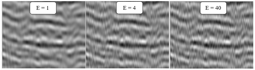
Fig.1 seismic image with different eigen values - 1, 4 ,40.
![]()
![]()
Skip - switch-off this module (do not use in the workflow).
Auto-connection - module is connected with previous (and next) modules in the workflow by default.
Bad data values option
There are 3 options for corrupted (NaN) samples in trace:
Fix - fix corrupted samples.
Notify - notify and stop calculations.
Continue - continue calculations without fixing.
Number of threads - perform calculation in the multi-thread mode.
![]()
![]()
Output gather - input seismic data minus random noise.
![]()
![]()
In this example we use a stack section as an input data and main goal is to attenuate random+linear noise.
Usually geophysics create these type of workflows on the poststack stage in order to remove remains of noise events after PSTM/PSDM procedures.
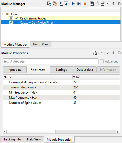
Fig.2 Workflow and module's parameters.
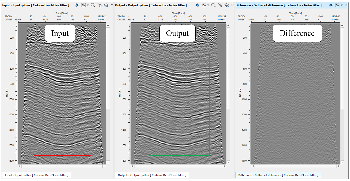
Fig.3 Stack section: before noise attenuation (left), after (middle) and difference (right).
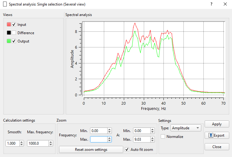
Fig.3 Amplitude frequency spectrum: before noise attenuation (red), after (green).
![]()
![]()
YouTube video lesson, click here to open [VIDEO IN PROCESS...]
![]()
![]()
Cadzow, J.A.: Signal enhancement—a composite property mapping algorithm. IEEE Trans. Acoust. Speech Signal Process. (1988)
Gillard, J.: Cadzow’s basic algorithm, alternating projections and singular spectrum analysis.
 If you have any questions, please send an e-mail to: support@geomage.com