Travel time tomography 3D/2D: depth velocity model updating (PSDM stage)
![]()
![]()
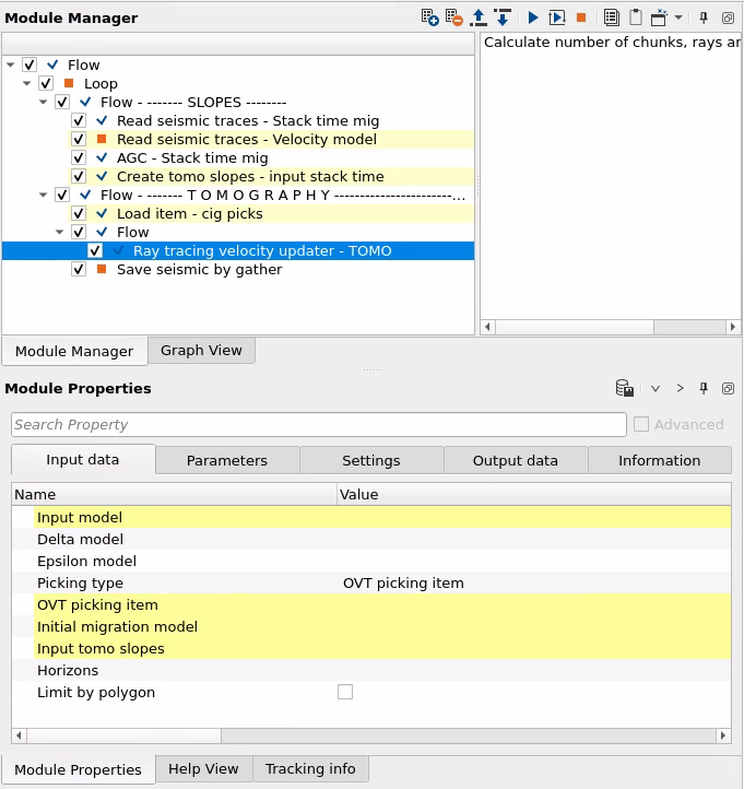
Ray tracing velocity updater module is a travel time tomography which is used for depth velocity model updating and it's included into the PSDM (Pre Stack Depth Migration) workflow: depth velocity model building 2D or 3D. The common scheme of the entire PSDM sequence you can fine in the example part of this documentation.
Ray tracing velocity updater produces modes of the subsurface P-wave velocity structure as well as of the geometry of energy reflecting boundaries. Velocity models are represented by independent 3D and 2D node meshes, respectively. These meshes are defined by the spatial coordinates of their nodes, each of which is given a specific parameter value.
3D traveltime tomography for the modeling of active source seismic data that uses the arrival times of both reflected seismic phases to derive the velocity distribution and the geometry of reflecting boundaries in the subsurface. The traveltime calculations are done using ray-tracing technique the graph. The LSCG algorithm is used to perform the iterative regularized inversion to improve the initial velocity and depth models. In order to cope with an increased computational demand due to the incorporation of the third dimension, the forward problem solver, which takes most of the run time, has been parallelized with a combination of multi-processing and message passing interface standards. This parallelization distributes the ray-tracing and traveltime calculations among available computational resources.
Steps:
1) Model parametrization
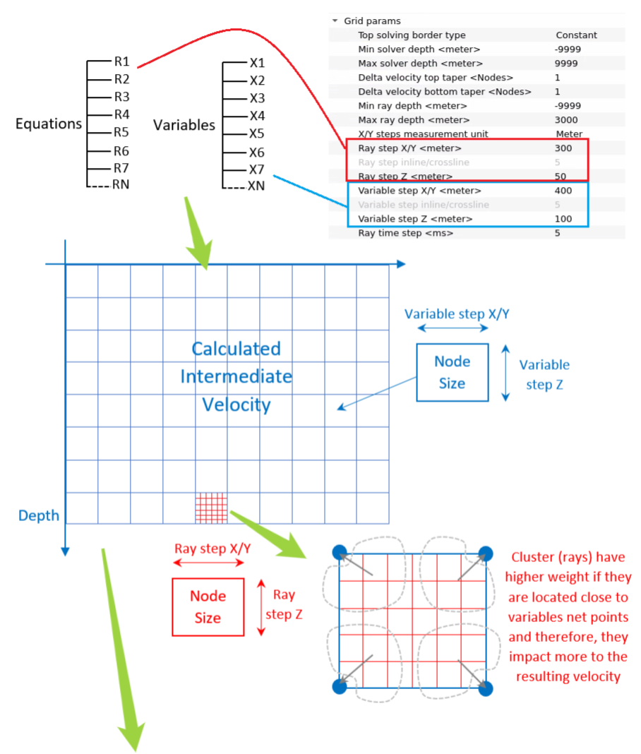
Module produces models of the subsurface P-wave velocity structure as well as of the geometry of energy reflecting boundaries. Velocity model is represented by 3D node meshes. These meshes are defined by the spatial coordinates of their nodes, each of which is given a specific parameter value. The spacing between nodes is cuboidal, and it should be finer than the smallest spatial size of velocity changes that the model is expected to account for. Each node in the mesh is assigned a value that corresponds to the P-wave velocity at that particular location in the subsurface. Each set of eight nodes defining a minimum-volume rectangular cuboid is called a cell. The velocity within each cell is found by trilinear interpolation of the eight nodes.
2) Forward problem
The forward problem is solved using a ray-tracing approach the graph method (Moser, 1991). The graph method, derived from network theory, calculates shortest paths through a discretized medium by connecting nodes within a predefined neighborhood (forward star, FS). It provides efficient initial estimates for reflected ray paths.
This approach balances computational efficiency and precision. The method’s flexibility allows it to adapt to varying model complexities, focusing computational effort only on nodes relevant to ray paths.
3) Inverse problem
Reflection (δt1j) travel time residuals for a given slowness (u=1/v, where v is velocity) and depth model are turned into parameter perturbations (δu and δz, respectively) following the integral equations for refracted (Г0i) and reflected (Г1j) ray paths:
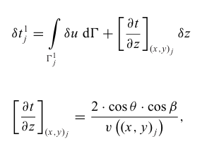
Where (x,y)j is the reflection point on the interface, θ is the incidence angle with respect to the interface normal vector, β is the local slope of the reflector, and v is the velocity at this point. Considering our discretization of the problem, previous equations can be collectively expressed in the following linear system:
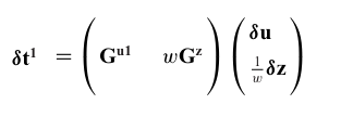
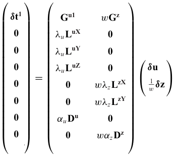
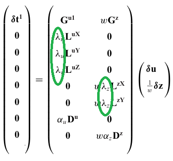
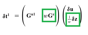
where δt1 is the vector reflection traveltime residuals, Gu1 and Gz are the Frechet derivative matrices (kernels) for velocity and depth, and δu and δz are the vectors of parameter perturbations. Each element in the velocity kernel is the length of the portion of a specific ray path partitioned to a relevant velocity parameter consistently with the trilinear interpolation. Typically, the number of available data is smaller than the number of model parameters, so the inversion of the previous equation is conducted with additional regularization constraints. The program works with three smoothing matrices for velocity perturbations (Lu), one for each direction as shown in the next equation.
These matrices are built with correlation lengths that can vary among nodes. The coefficients λu and λz determine the relative importance of smoothing with respect to data fit and are selected empirically:
![]()
![]()
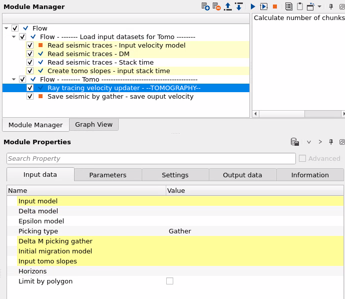
Input model - Input velocity model 2D or 3D is a migration model/wells model or also may be an output velocity model from tomo updating (from this module) and used as Input model for the next tomo updating (without doing seismic migration and DM/CIGs picking). Format is velocity traces (2D section or 3D cube) in depth domain on the constant datum (trace headers SOURCE_DATUM, RECEIVER_DATUM should be checked). Usually, this velocity can be get from time migration step (after Map migration procedure) and converted into interval velocity via Dix module.
Delta model - Input Delta model 2D or 3D (optional). Thomsen Delta attribute is produced by the PSDM imaging module (well-tie option).
Epsilon model - Input Epsilon model 2D or 3D (optional). Thomsen Epsilon attribute is produced by the VTI epsilon estimation module.
Picking type :
Gather - use this type in case input velocity/misfits picking is DM (delta misfits) gathers (in traces).
DVrms picking item - use this type in case input velocity/misfits picking is DM (delta misfits) item (internal g-Platform format).
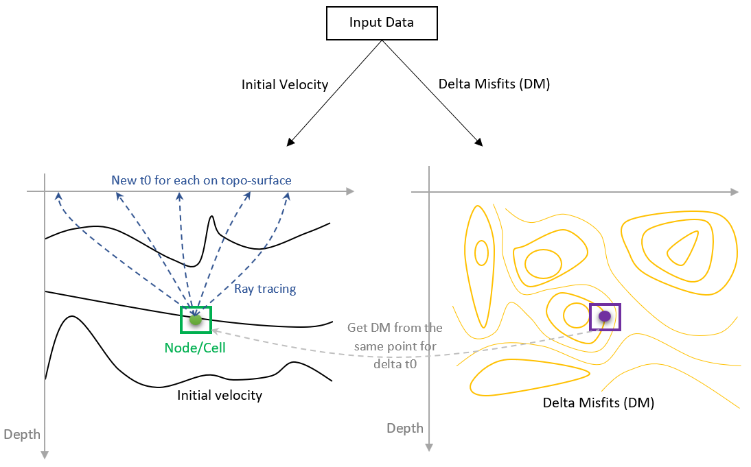
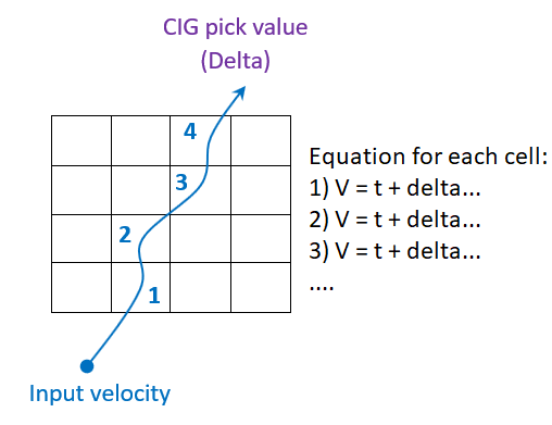
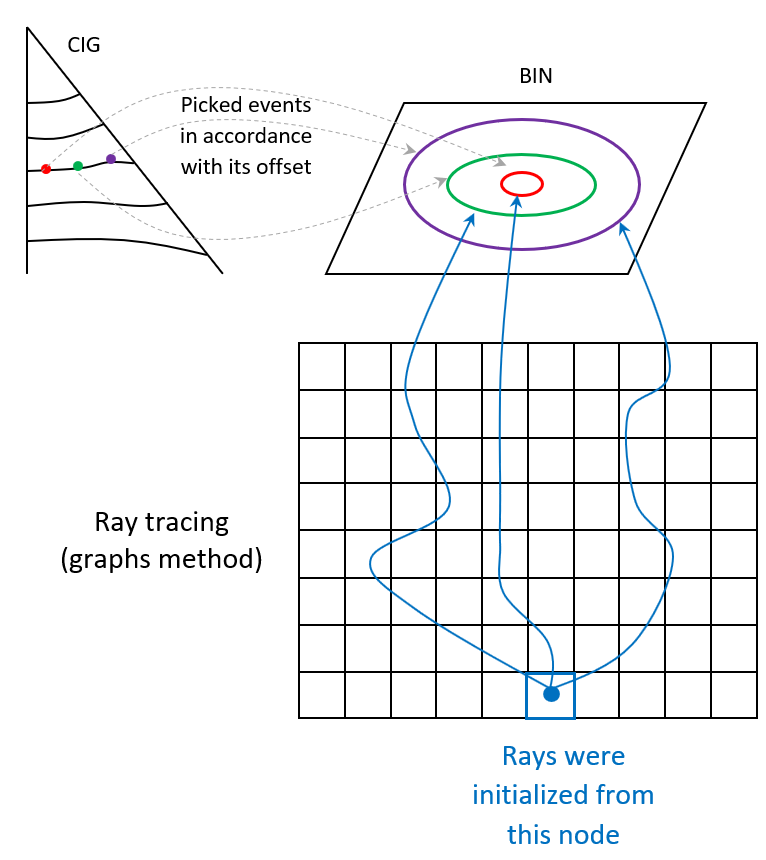
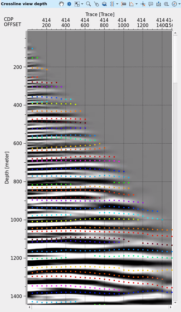
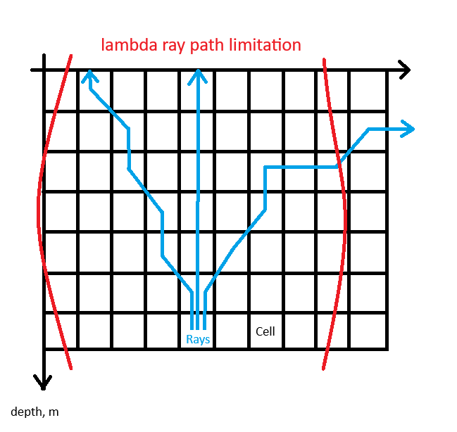
OVT picking item - use this type in case input velocity/misfits picking is CIG picks (Common Image Gather picking events for each offsets) item (internal g-Platform format). CIG picking (signal event) is performed on each offset on the common image gather, then this picking is used for calculation of new (edited) velocities via cell-tomography. Quantity of cells depends on quantity of picks: less picks, less solution density. On each node (cell), example on the picture below, highlighted by blue, there is an initialization of ray tracing via input velocity model (initial), up-to trough all nodes which are located on the way. Ray density is defined by tomography parameters, each ray come to some picked event (pic. highlighted by red, green, purple). After obtaining the Delta t value from picking at a particular location (Delta t = t0 - t current), we can recalculate the velocity model using a system of equations. This system represents the desired velocity model at each node through which the ray passed. On output there is a corrected velocity model in accordance with CIG picks:
Delta M picking gather - delta M picking gathers. Can be produced by PSDM imaging module after delta velocity spectrum picking.
Delta Vrms picking item- delta M picking item (internal g-Platform format). Can be produced by PSDM imaging module after delta velocity spectrum picking.
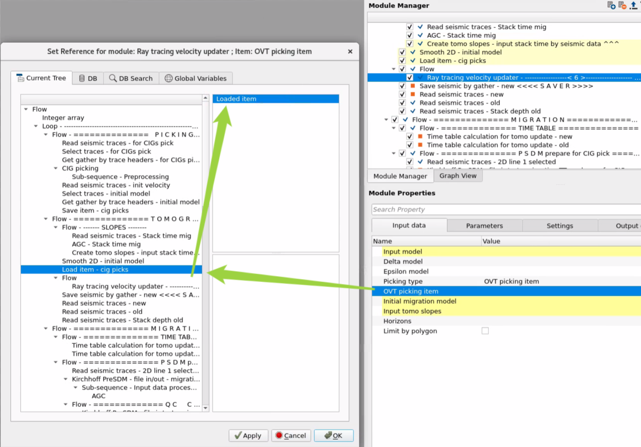
OVT picking item- Common Image Gather picking events for each offsets (CIG picks) item (internal g-Platform format). Can be produced by CIG picking. Example of item connection:
Initial migration model - Input migration velocity model 2D or 3D is a model which was used for gather migration process (PSDM).
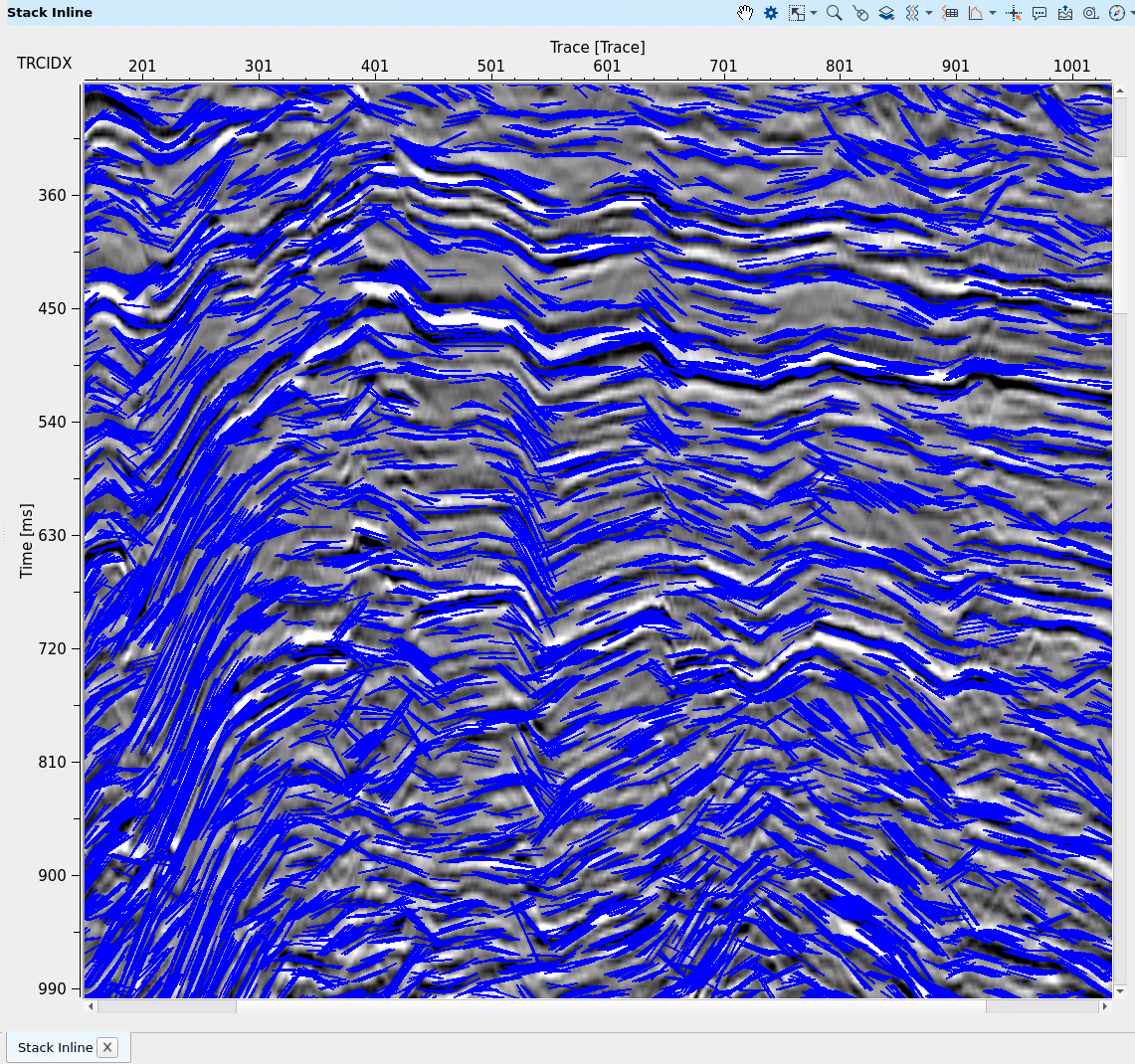
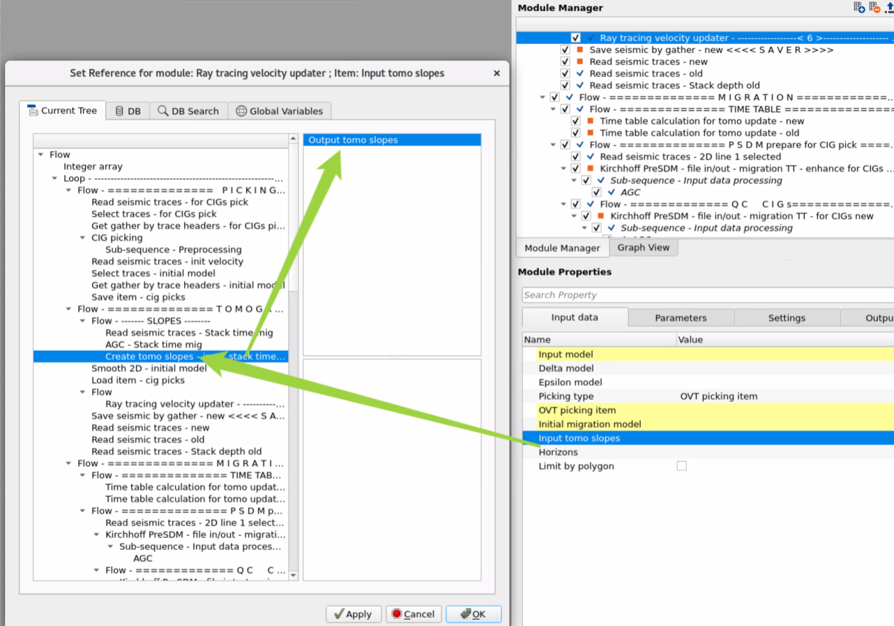
Input tomo slopes - stack slopes are used (optionally) as velocity constrain, it's produced by the Create tomo slopes module. The slopes make an output model be more geologically consistent, i.e. velocity will be in accordance with horizons/layers. This input data is highly recommended to use. Example of slopes, Stack section (gray scale) + slope picking (blue):
Example of item connection:
Horizons - input horizons are used for velocity smoothing, i.e. tomo parameter Smooth will use it. Optional, by default smooth works in accordance smooth aperture: horizontal and vertical.
Limit by polygon - we can use limitation for calculations by XY polygon. Prepare picking polygon before tomography process and use it for tests or limited area calculation.
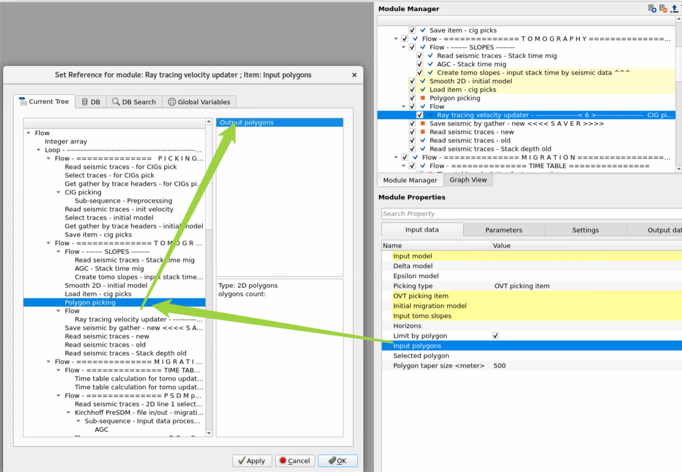
Input polygons - define input polygon via selection from the Polygon picking module like on the example below:
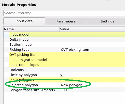
Selected polygon - the list of polygons is available after previous step. By default the first picked polygon is selected:
Polygon taper size - taper for polygon borders in meters.
![]()
![]()
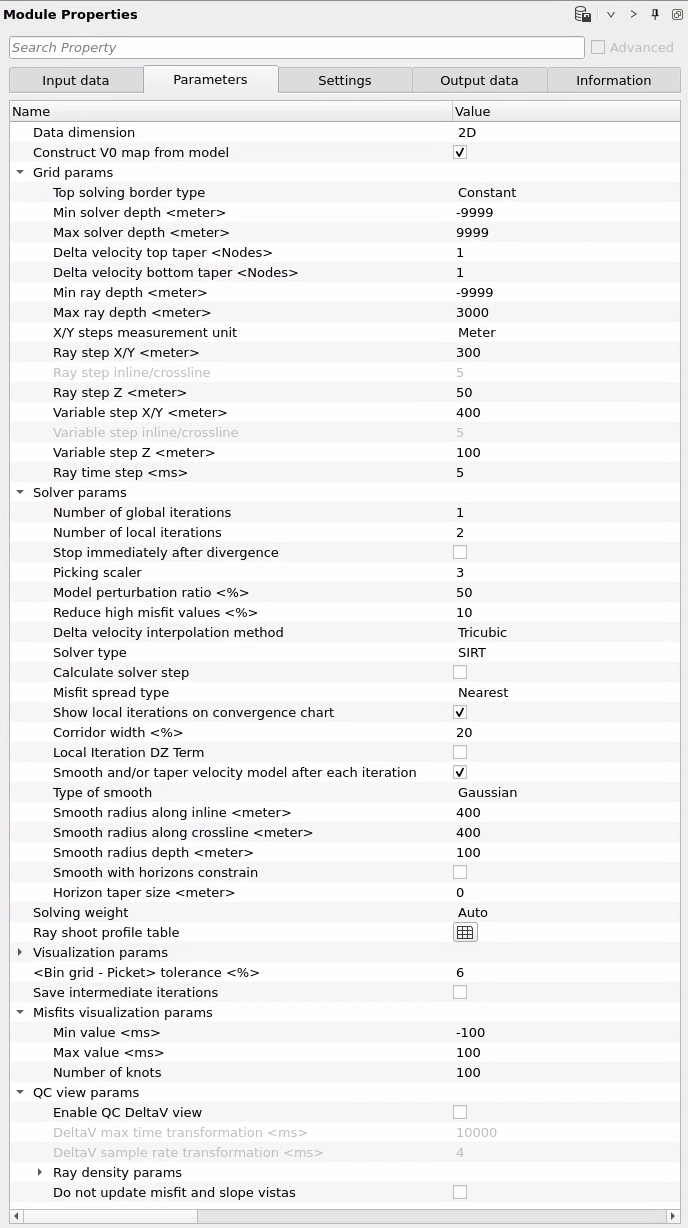
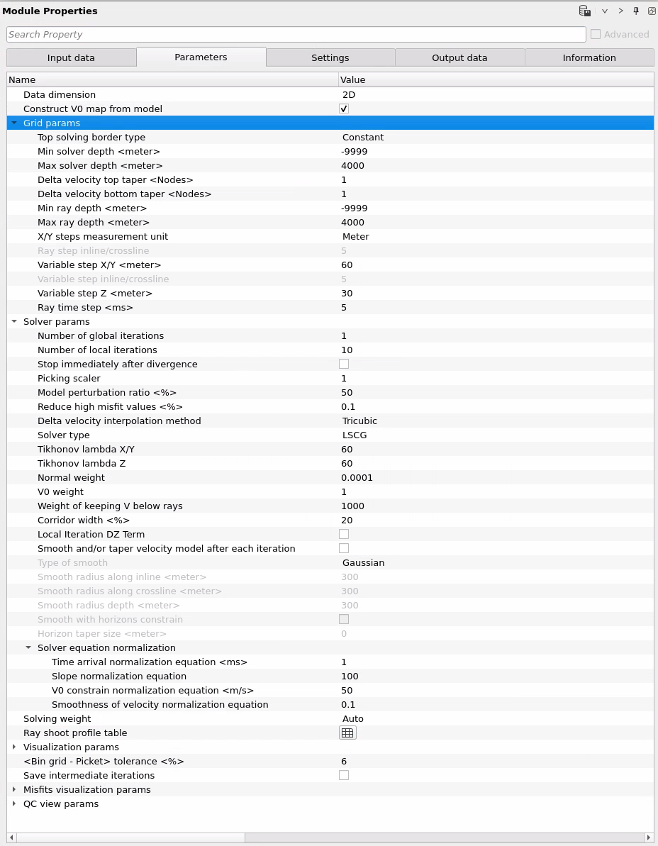
Data dimension { 2D, 3D } - select type of input data 2D or 3D. This option is for ray shooting and it saves time for calculations.
Construct V0 map from model - V0 gets from the first sample of the input velocity.
V0 - If option is Enabled: V0 map constructs from input velocity model, if Disabled: user should define velocity V0 value manually.
Grid params - tomography grid/cell definition:
Top solving border type - two types for start layer for solve calculations:
Constant - solving starts from defied constant depth.
Horizon - solving starts from this horizon.
Min solver depth - start depth in meters for start solve calculations.
Top solving horizon - select horizon from the list (must be loaded in Input params tab) which will be user as start layer for solver calculations.
Max solver depth - stop depth line in meters is for stopping solve calculations.
Delta velocity top taper - taper in nodes (cells) is for top (start line) velocity merge line.
Delta velocity bottom taper - taper in nodes (cells) is for bottom (stop line) velocity merge line.
Min ray depth - minimum depth in meters is for ray path initialization start position (there is no ray calculation above).
Max ray depth - maximum depth in meters is for ray path stop position (there is no ray calculation below).
X/Y steps measurement unit - X and X units format for variables and steps below: in meters or Inline&Crossline.
Ray step X/Y - definition for horizontal ray path grid is in X/Y, meters.
Ray step inline/crossline - definition for horizontal ray path grid is in Inline&Crossline.
Ray step Z - definition for vertical ray path grid is in X/Y, meters.
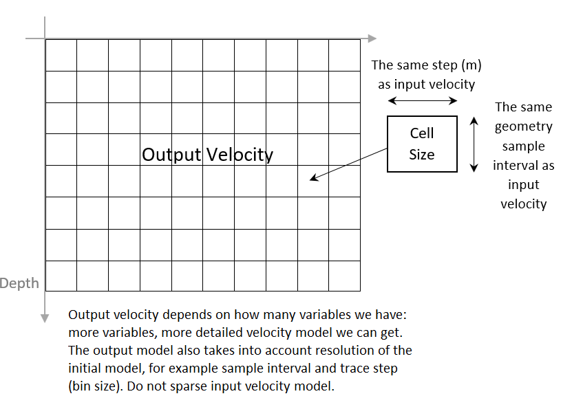
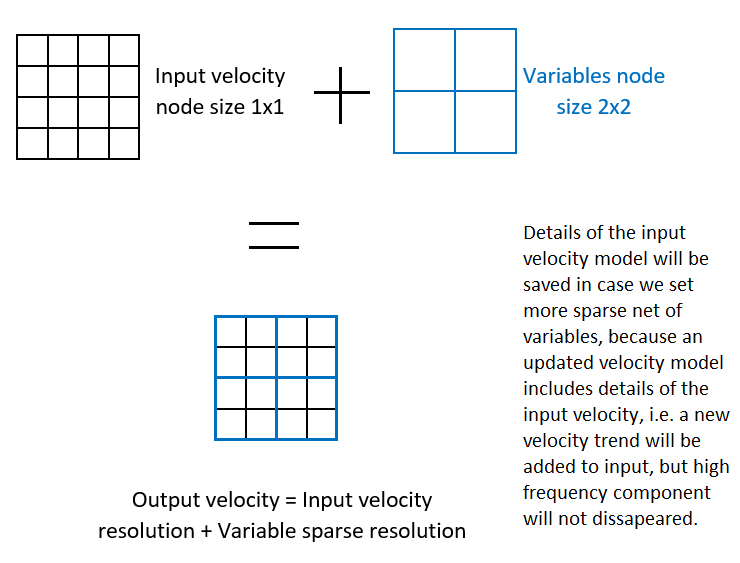
Variable step X/Y - definition for horizontal output velocity grid is in X/Y, meters. Velocity resolution (horizontal).
Variable step inline/crossline - definition for horizontal output velocity grid is in Inline&Crossline. Velocity resolution (horizontal).
Variable step Z - definition for vertical output velocity grid is in X/Y, meters. Velocity resolution (vertical).
Ray time step - definition for vertical ray path grid is in X/Y, milliseconds.
Solver params
Number of global iterations - number of iteration or one of selected algorithms: LSQR, LSCG, SiRT, Mean.
Number of local iterations - solution, number of iteration inside 1 global iteration of LSQR, LSCG, SiRT, Mean. Error minimization process. Number of local iteration must be proportional to quantity of variables, i.e. we can you the following equation for local iteration calculation: (( model depth / step Z variable ) * line length / step X/Y ) * 2 , line length means 2D seismic profile, or we can use inline/crossline length for calculation.
Stop immediately after divergence - stop calculations if the previous error is less than current one. For example, we have defined 10 global iterations, but after the 2-nd iteration module stopped calculation, so eventually we have solution after two global iterations.
Picking scaler - temporary parameter, excremental!!! it depends on picking: if input is DM then we should use scaler = 3-4, if CIG picks - do not use scaler (use = 1), !!!IMPORTANT please do tests 1, 2, 3, 4 for DM.
Model perturbation ratio - percentage of velocity model changes that are allowed from it's input values.
Reduce high misfit values - this parameter is for removing outfits of ray errors. Values: 0-100%.
Delta velocity interpolation method { Trilinear, Tricubic } - need for performing conversion of the Velocity grid variables into velocity model resolution (i.e. input velocity gather parameters (SI/Trace length).
Solver type { LSCG, LSQR on CPU, LSQR on remote GPU, Mean value, Mean value (distributed), SIRT } - solve computation, local iterations:
LSCG - least square conjugate gradient (standard mathematical method can be found from publicly available sources).
LSQR - least square QR decomposition (standard mathematical method can be found from publicly available sources).
SiRT - simultaneous iterative reconstruction technique (standard mathematical method can be found from publicly available sources). Faster solution, less time consuming algorithm.
Mean value - similar to SiRT, it should be remove in the next versions. LSCG/LSQR vs Mean: for the LSCG/LSQR we should to tune Tikhonov parameters in order to remove velocity anomalies "bull-eye effect", but in the Mean method there is no Tikhonov, but there is a smoothness parameter. Also, Mean method is slower in terms of convergence. In the Mean method we need to check a density of rays, it should be less than 100 for each node (have a look at output QC file of rays), to avoid low fold (10 for example). For example, if parameter of node size tomography (ray step) equal 100 meters, then step of variable equal 50 meters.
Calculate solver step - coefficient is automatically calculated for faster convergence.
Misfit spread type { Nearest, Spline, Gaussian } - when misfit (milliseconds) is converted/solved into velocity grid this interpolation process is used: Nearest, Spline, Gaussian interpolation type. Recommendation: use Nearest.
Show local iterations on convergence chart - show local graph on the visual Vista Item, if necessary.
Tikhonov lambda X/Y - constrain horizontal smooth aperture (meters) is used for ray path limitation/stabilizing. The result is less fluctuated on the output velocity, there is less "Bull-eye" artifacts/effects on the output velocity, so we can remove velocity anomalies on the output velocity model by this parameter. Important! higher lambda , solution will be simpler therefore it will be easier or convergence, caused by smooth model. Tikhonov lambdas are in the reverse problem equation:
Tikhonov lambda Z - constrain vertical smooth aperture (meters) is used for ray path limitation/stabilizing.
.
Normal weight - weight parameter is for slopes constrain: values from 0 to infinity (0 - no slope using).
V0 weight - weight for V0 (from 0 to infinity), if high value defined, it means that an algorithm keeps V0 velocity the same as it was (does not change it).
Weight of keeping V below rays - parameter is for the depth's keeping or changing interval after Max ray depth limit: i.e. if needed to change it or not. (0 - infinity). If high value, it means that velocity below will be saved (keep original velocity).
Corridor width - limitation in percentage of the velocity changing (% constrain).
Local Iteration DZ Term - for SiRT algorithm, inside the solver we switch ON auto-recalculate reflection point shift
Smooth and/or taper velocity model after each iteration - apply smoothing procedure on velocity model after each update.
Type of smooth { Usual, Gaussian, None } - select a type of smoothing procedure on velocity model after each update.
Smooth radius along inline - smoothing aperture in meters along Inline direction only.
Smooth radius along crossline- smoothing aperture in meters along Crossline direction only.
Smooth radius depth- smoothing aperture in meters vertical direction only.
Smooth with horizons constrain - in case we have horizons on input this option does smoothing in accordance with horizons.
Horizon taper size - in case we have horizons on input this option does taper for smoothing in accordance with horizons.
Use thick rays - delta velocity conversion/distribution by the Nearest interpolation method (if disabled) and B-spline (if enabled).
Cell weight threshold - recommendation: not to use it. Experimental. Weight for removing outfits of bad cells (cell without rays low fold).
Solving weight:
Ray weights table
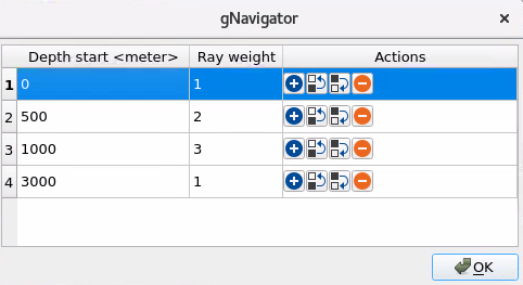
Manual - flexible table depth/weight user can define manually, it means that higher weight will lead to make ray path solution more solid (i.e. don't change this path (node), but use node as true path of the ray distribution). We can "freeze" upper part of the model, for example a depth interval 0-500 meters by defining a weight = 1, but for the deeper part define weight = 100000 (not higher because it does not make sense, i.e. will not enough accuracy of solution).
Auto - depth/weight set automatically by exponent function: top - low weights , bot - high weights.
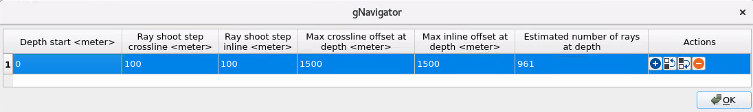
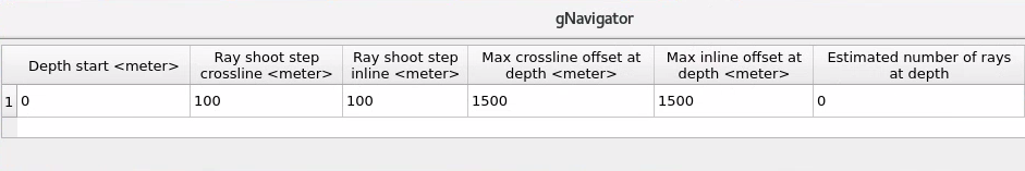
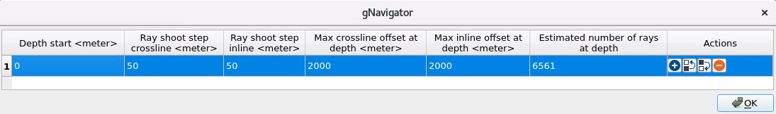
Ray shoot profile table - a flexible table for rays initialization (shooting) parameters, i.e. how dense or sparse it should be:
For particular depth we can define step inline and crossline direction step, maximum offset. One row can be used for the entire depth section, or several rows of definition which will be interpolated between. Also there is an information column where we can fine estimated number of rays at depth. Large number of ray leads to time consuming calculations, but more accurate, so we should find a compromise:
Visualization params - these set of parameters are only for visualization different Vista for QC.
Inline to show - exact Inline number for visualization. Use it in case of 3D data set, otherwise if 2D there is no need to define it, 2D line will be appeared automatically.
Crossline to show- exact Inline number for visualization. Use it in case of 3D data set, otherwise if 2D there is no need to define it, 2D line will be appeared automatically.
Layer width - what the distance from Inline/Crossline point should be an image point to create a visual vista item image.
<Bin grid - Picket> tolerance - for all input data (Vel, picks, ect.) checking pickets that they are correct/consistent. Do not change this auto parameter.
Save intermediate iterations - if this option is enabled module will save every velocity model of all Global iterations. By default there is only last velocity model on the output from the module.
Intermediate iterations params - path for intermediate velocity models.
File name - velocity model name.
Prefix - prefix for velocity model.
Misfits visualization params - visual Vista Item for QC:
Min value - minimum misfit for visualization in milliseconds.
Max value- maximum misfit for visualization in milliseconds.
Number of knots - how many groups are separated on the Misfits distribution graph.
QC view params:
Enable QC DeltaV view - switch on Delta V visual Vista Item for QC.
DeltaV max time transformation - maximum time transformation in milliseconds for viewing on Vista Item.
DeltaV sample rate transformation- minimum time transformation in milliseconds for viewing on Vista Item.
Ray density params: possibility to save extra QC attributes
Ray density volume - file name for output image points, color means count of rays for this point.
Ray density volume full trajectory path - file name for output ray's fold (depends on weights) for every node/cell.
Interpolation aperture - parameter in meters for performing an interpolation process to create QC attributes.
Do not update misfit and slope vistas - switch ON/OFF visual Vista Items updating during calculations.
![]()
![]()
Execute on { CPU, GPU } - select which type of processor will be used for calculations: CPU or GPU.
Distributed execution - if enabled: calculation is on coalition server (distribution mode/parallel calculations).
Bulk size - chunk size is RAM in megabytes that is required for each machine on the server (find this information in the Information, also need to click on action menu button for getting this statistics):
Limit number of threads on nodes - limit numbers of of threads on nodes for performing calculations.
Job suffix - add an job suffix.
Set custom affinity - an axillary option to set user defined affinity if necessary.
Affinity - add your affinity to recognize you workflow in the server QC interface.
Number of threads - limit number of threads on main machine.
Run scripts - it is possible to use user's scripts for execution any additional commands before and after workflow execution:
Script before run - path to ssh file and its name that will be executed before workflow calculation. For example, it can be a script that switch on adn switch off remote server nodes (on Cloud).
Script after run- path to ssh file and its name that will be executed before workflow calculation.
Skip - switch-off this module (do not use in the workflow).
![]()
![]()
Output model - resulting (final) velocity model after tomography updates.
Delta V - Delta velocity for QC purposes ( Delta = V input - V output).
Delta V normalized- Normalized delta velocity for QC purposes.

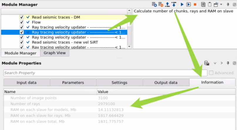
Number of image points
Number of rays
RAM on each slave for models, Mb
RAM on each slave for rays, Mb
RAM on each slave total, Mb
![]()
![]()
Calculate number of chunks, rays and RAM on slave - provides useful information for server (coalition) distribution execution that we can find in the Information tab after clicking on this action button:
![]()
![]()
Some common rules for tomography parameters:
- quantity of variables should be more then equations, otherwise resulting solution would be not stable. An example of incorrect parameters:
Ray step X/Y=100, Ray step Z = 100, bit Variable step = 10, Variable step Z = 10, in this case we have large ray node(cell) and small nodes of variables.
- we should start with relatively big cluster (node/variable sizes) to have enough smoothness for velocity model, so it's more stable on first iterations (first steps). For example, Ray step X/Y= 800 m, Ray step Z = 400 m, variables must be in 2-3 time bigger: Variable step X/Y=1600 m, Variable step Z = 800 m.
- in each next iteration make ray steps (node size) less, at the same time keep a variable node size in a few times bigger: Ray step X/Y=100 m, Ray step Z = 25 m, Variable step X/Y = 400 m, Variable step Z = 150 m.
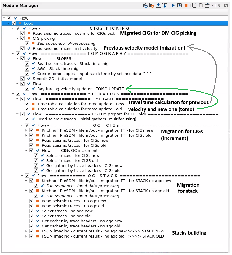
Example of a workflow in case of DM picking. The First update:
!!! Important: to make an examples easier for understanding this part of the flow is only for tomography process, therefore you have to do a DM picking before and calculate Time Tables (travel times) for depth migration, after that you can perform depth migration and see common image gathers and build a stacks before and after tomo update. You can find full workflow in the end of the example chapter.
Ray shoot profile table:
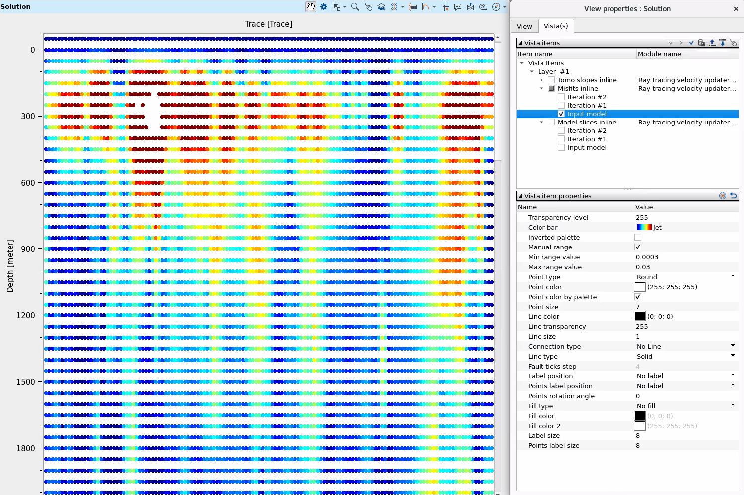
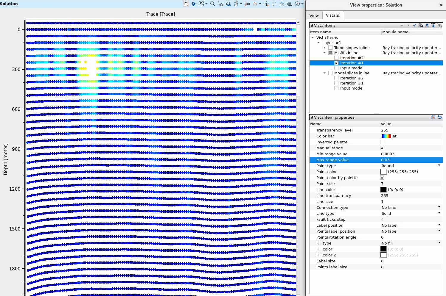
QC errors visualization (misfits depend on the input DM picking gather, see it also for QC):
High values on the initial then become smaller after 1 update
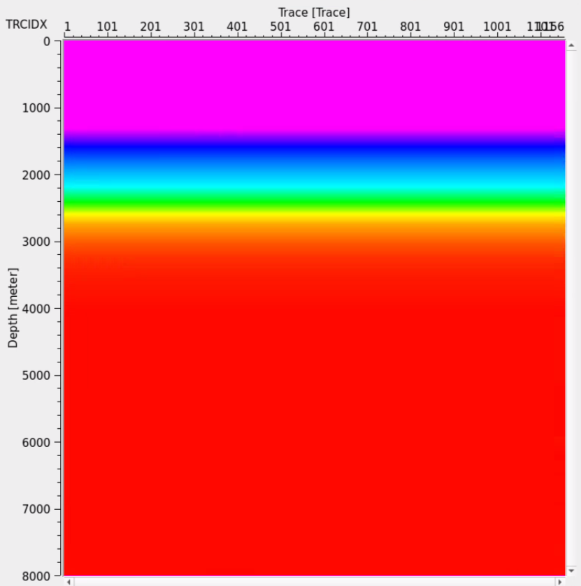
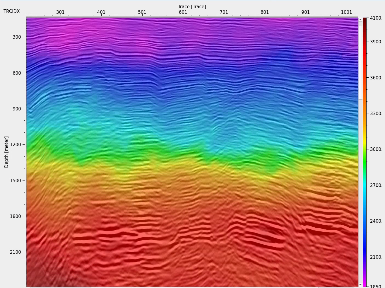
Input background velocities:
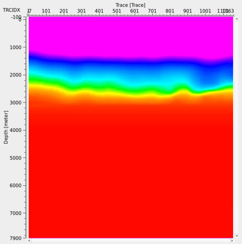
Output first update tomography velocities (smooth fluctuations):
Convergence graph:
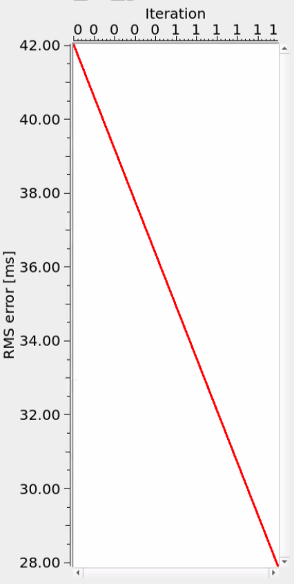
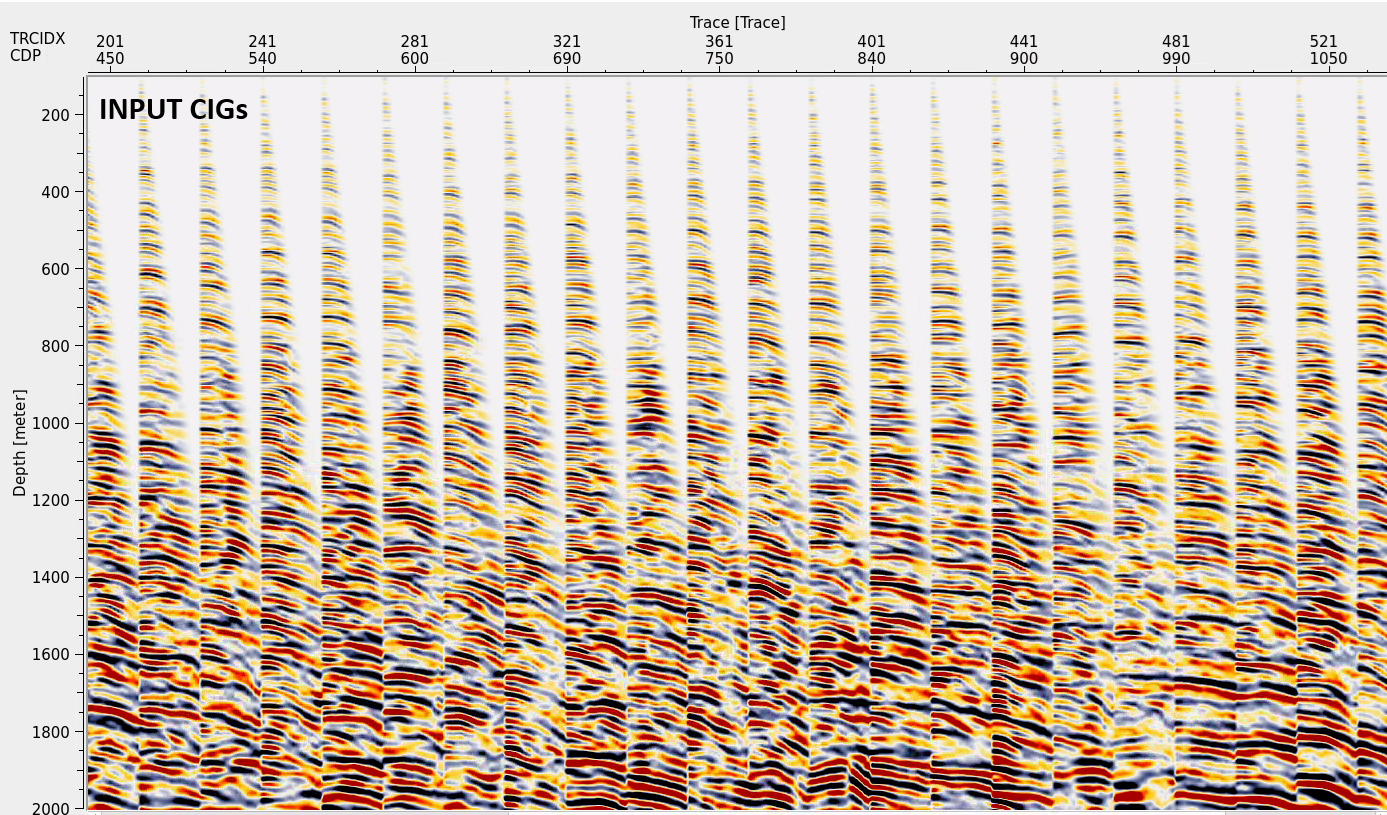
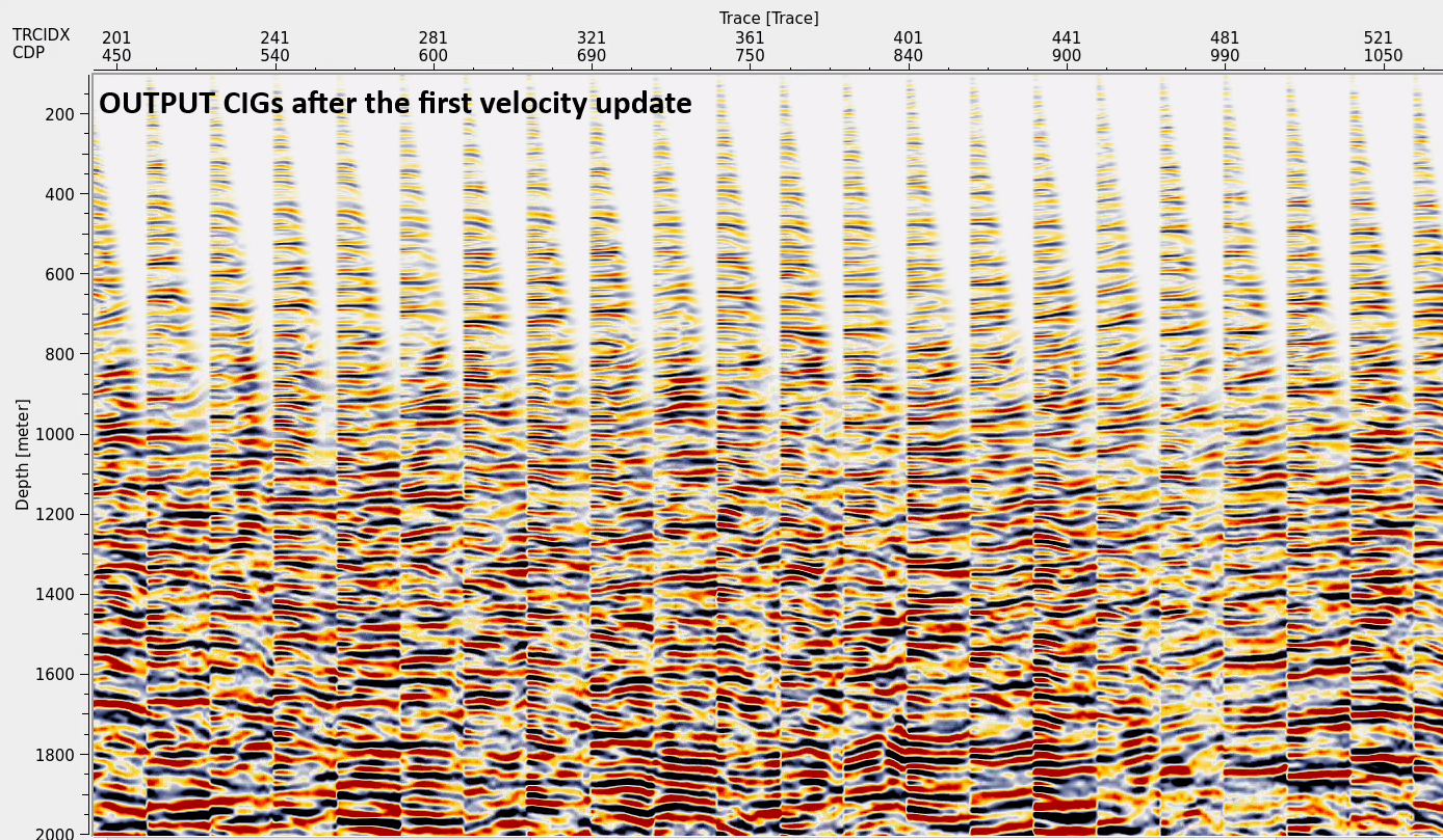
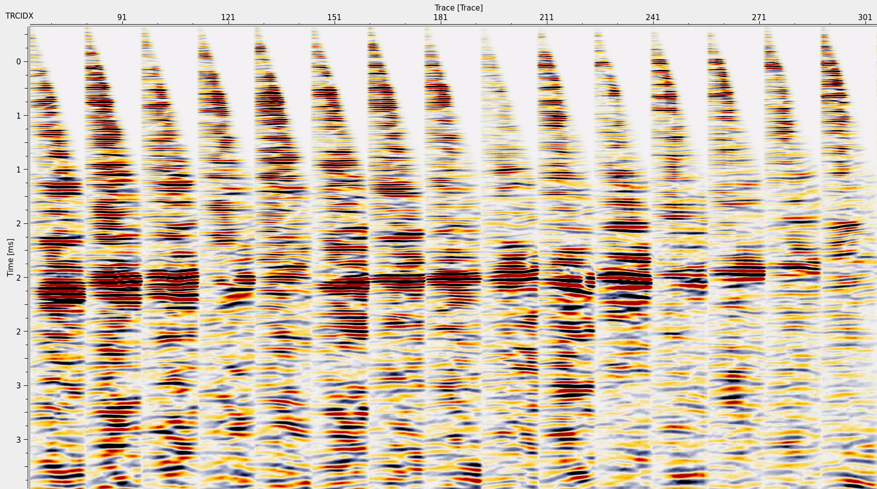
CIGs before and after the first tomo update:
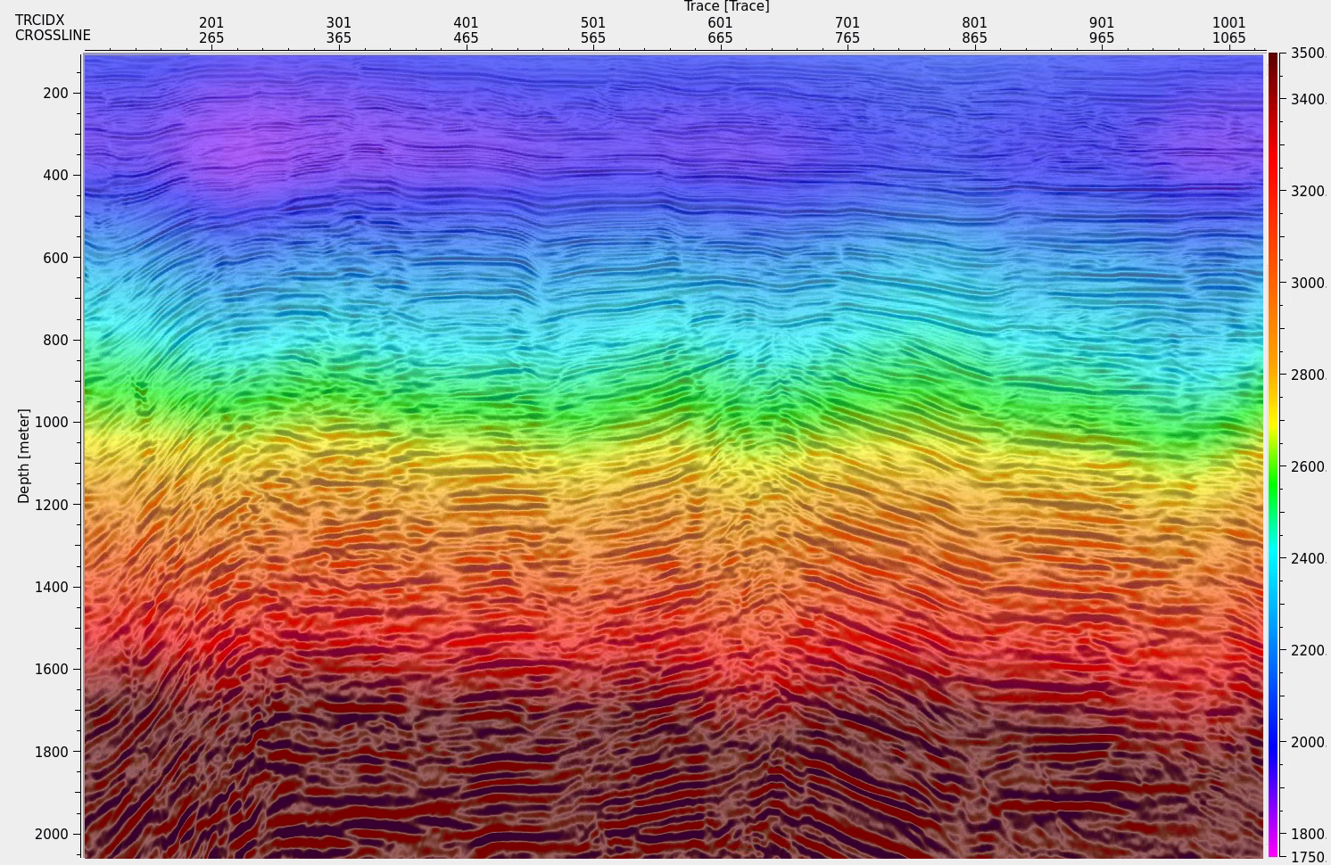
Output velocity model:
Example of a workflow in case of CIG picking. The last 6-nth tomo update:
Example of the full workflow with all necessary calculation, input picking and output QC data-sets. We can split this flow into several separated workflows if it necessary:
Input CIG picks example for the one CIG. Different color means that events belongs to one particular reflector (different color, different reflectors):
Ray shoot profile table:
Final detailed velocity model after 6 tomo updates (2 first were used DM picking, others CIG picks):
CIGs in time after the last 6-nth tomo update:
![]()
![]()
TOMO 3D: 3D joint refraction and reflection traveltime tomography parallel code for active-source seismic data—synthetic test A. Mel´endez, J. Korenaga, V. Sallar`es, A. Miniussi and C.R. Ranero.
 If you have any questions, please send an e-mail to: support@geomage.com