Binning of a 3D seismic data

Theory

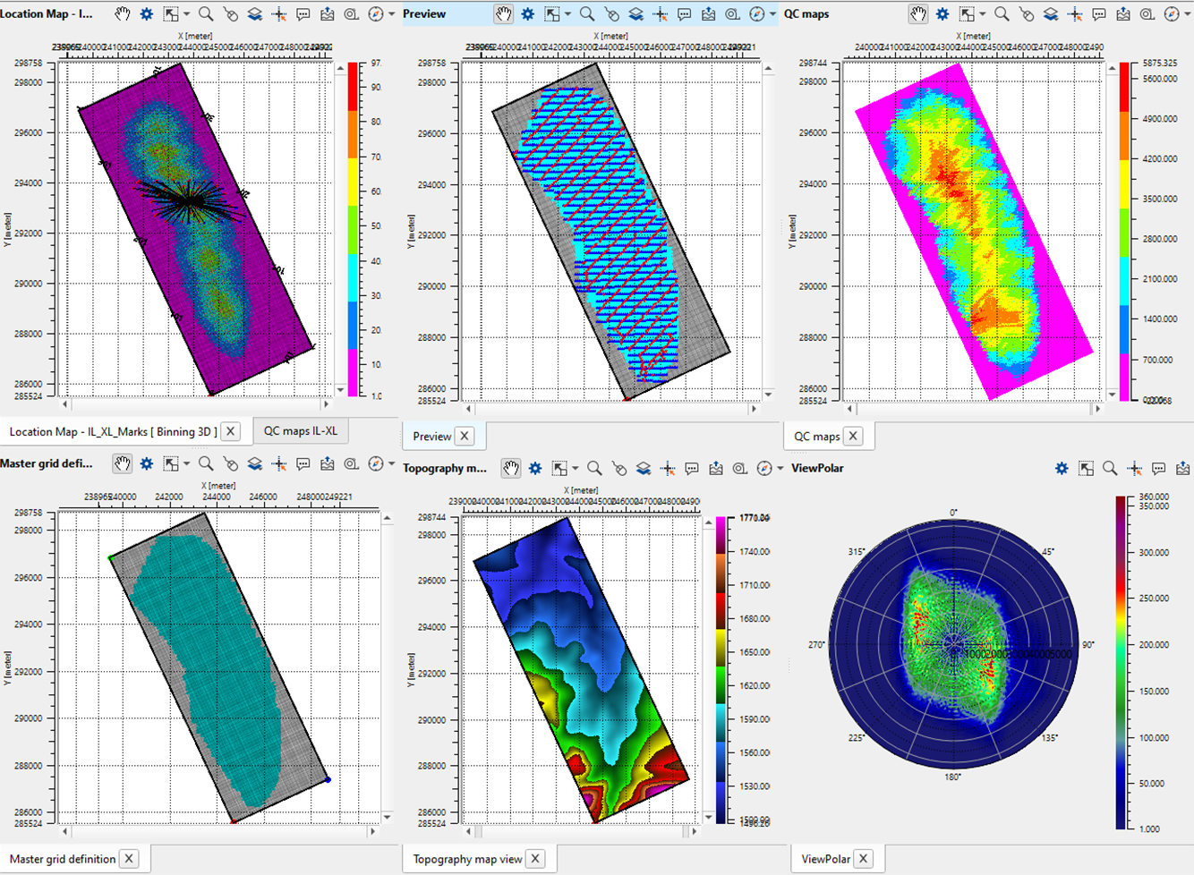
This module performs binning for 3D seismic data, the input data are seismic traces with geometry updated to the trace headers. (Source and receiver X,Y,Z coordinates and station numbers). Binning 3Dcreates a smoothed topography surface (CMP) using user specified parameters and saves it to the trace headers for use with MultiFocusing and velocity analyses.  It also produces an unsmoothed version of the topography as well. The module produces several other QC’s to check the positioning of the grid bin centers relative to the midpoints in a bin. Other QC’s generated and available as Vista views are a fold of coverage map, minimum and maximum offset distance in a bin, bin center to bin centroid distance, bin center to bin centroid distance of X and Y coordinates, a rose diagram giving some azimuthal information, statistical information about the grid (the number of inlines, crosslines, size of area, etc.), a source/receiver midpoint/bin center location map as well as the bin topography map (smoothed and unsmoothed).

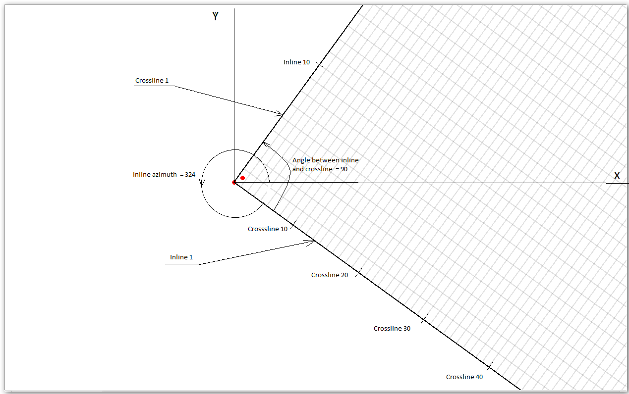
How to create/edit a master bin grid definition?

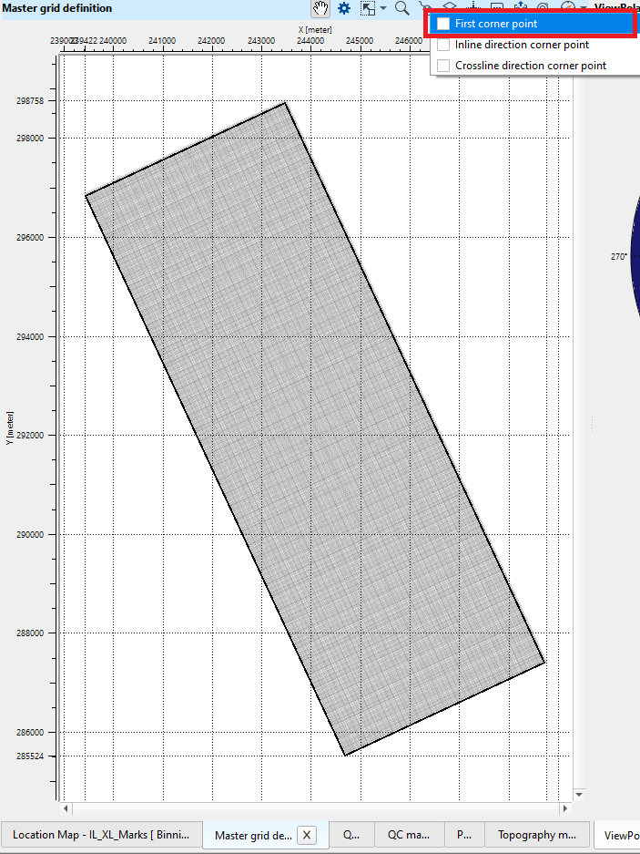
In case the user wants to create a bin grid or want to edit the existing bin grid, it can be done with manual editing of the Master grid definition window. Open the Vista Items of the Binning 3D module and go to Master grid definition window.

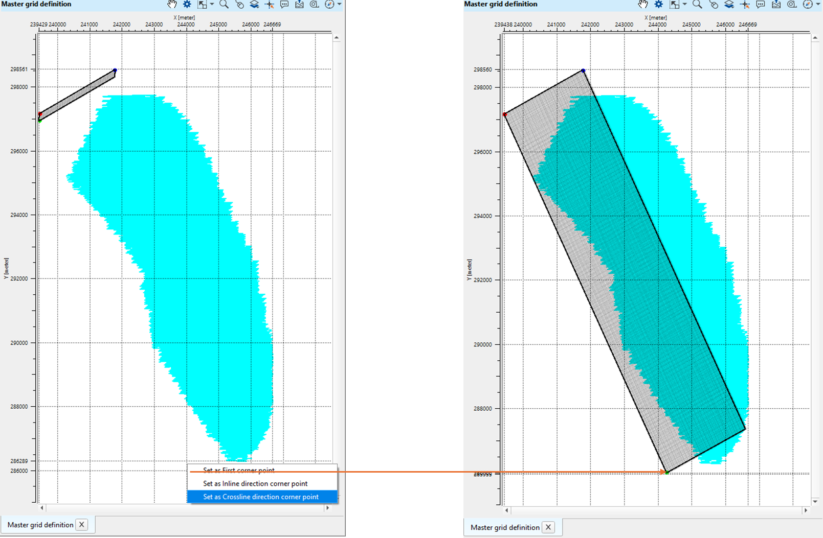
1. Go to Control items and select/check the first cornet point option

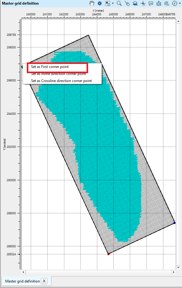
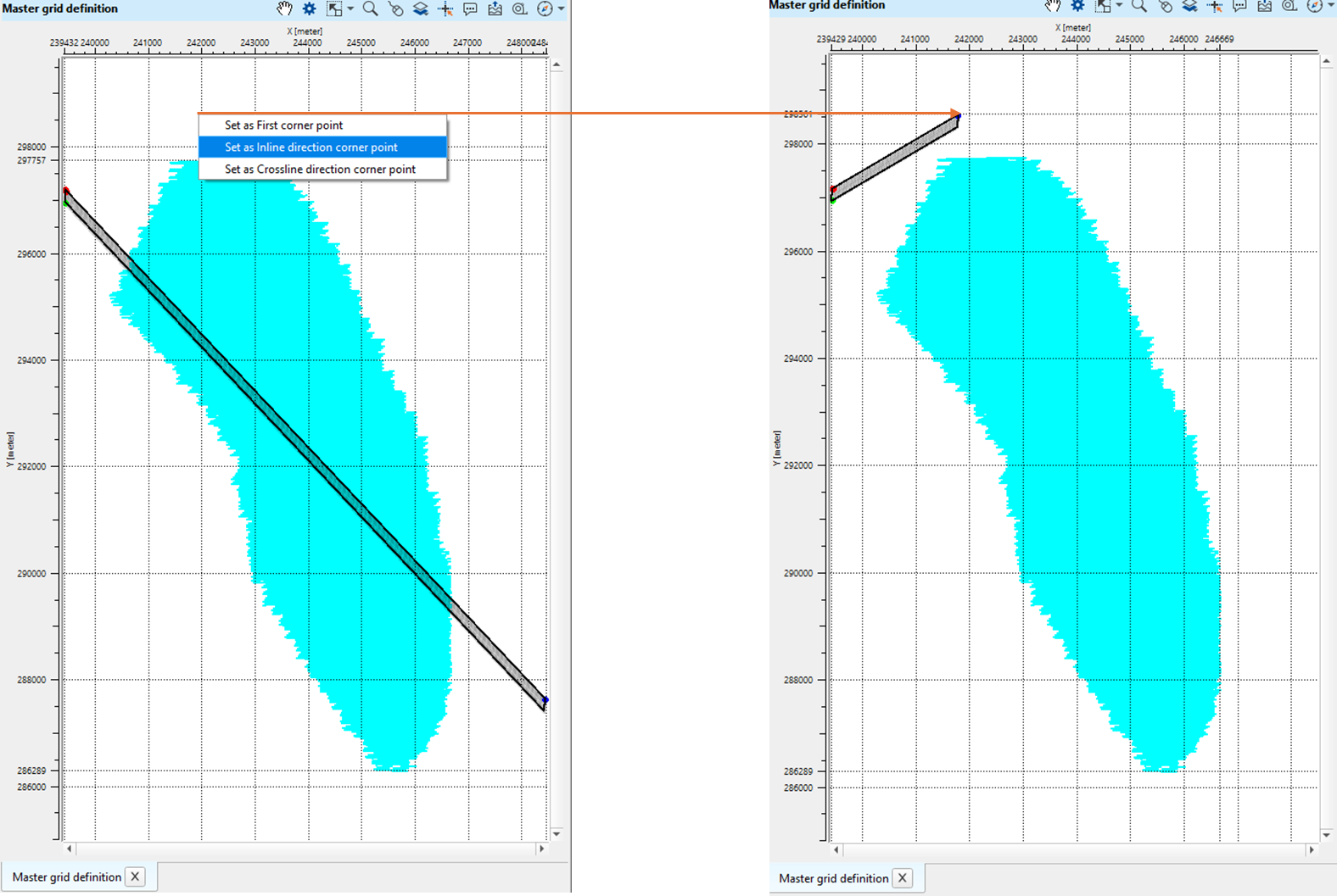
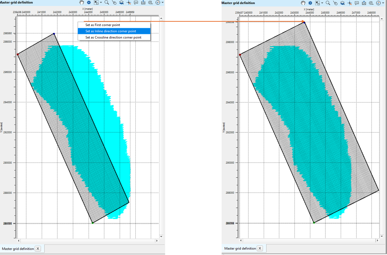
2. Go to the area where the user wants to set the grid starting point and click Alt+Right Mouse button (Alt+MB3) on the Master grid definition map and select "Set as starting point". If the master grid definition information is already existing like the one we've shown in the example then it will change the grid configuration.

3. Next, select/click on Inline direction corner and proceed as described in the step 2.

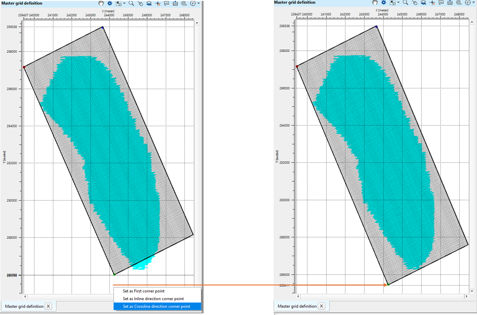
4. Likewise, select/click on Crossline direction corner point and proceed as described in the step 2.

If you look at the final master grid definition window, Mid Points are outside the bin grid. In order to put all the Mid Points inside the bin grid, the user should adjust/change the positions of the starting corner points, inline and crossline starting points to make sure all the Mid Points are falling inside the bin grid.

To adjust/change the starting corner point and/or first inline cornet point and/or crossline cornet point, go to that particular area and follow the same procedure as described in the steps 2,3,4 and adjust the points.

This exercise is an example demonstration to showing how to edit an existing master grid definition file or to create a new master grid definition file.

Input data

Input DataItem

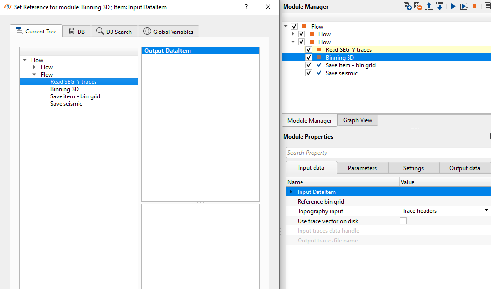
Input trace headers

connect/reference the input trace headers. This can be dependent on the kind of input data we've in the workflow. In case the input data is raw data then we need to provide the Output trace headers of Geometry application module. In case the input data trace headers are already having geometry information, we can simply provide the output trace headers from the "Read SEG-Y traces" module.

Reference bin grid

Provide the reference bin grid if any

Connect this input to the Output bin grid from a previously executed Binning 3D module, or from any other module that produces a bin grid object, when you want to replicate an existing grid geometry. When a reference grid is connected and the Recalculate bin grid by reference grid custom action is invoked, all grid definition parameters (origin, azimuth, inline/crossline numbers, and bin spacings) are automatically populated from the reference. This is useful when processing multiple vintages or datasets that must share a common bin grid, or when reprocessing a subset of data that must align with the master survey grid.

Topography input { Trace headers, Sources and receivers collection, External file, External map, Marine data }

There are various options available to get the topography (elevations) information to generate the topography maps, updating the trace headers for the newly formed bins.

TopographyInput - Trace headers

This is the default option which means it will automatically takes the topography information from the input trace headers.

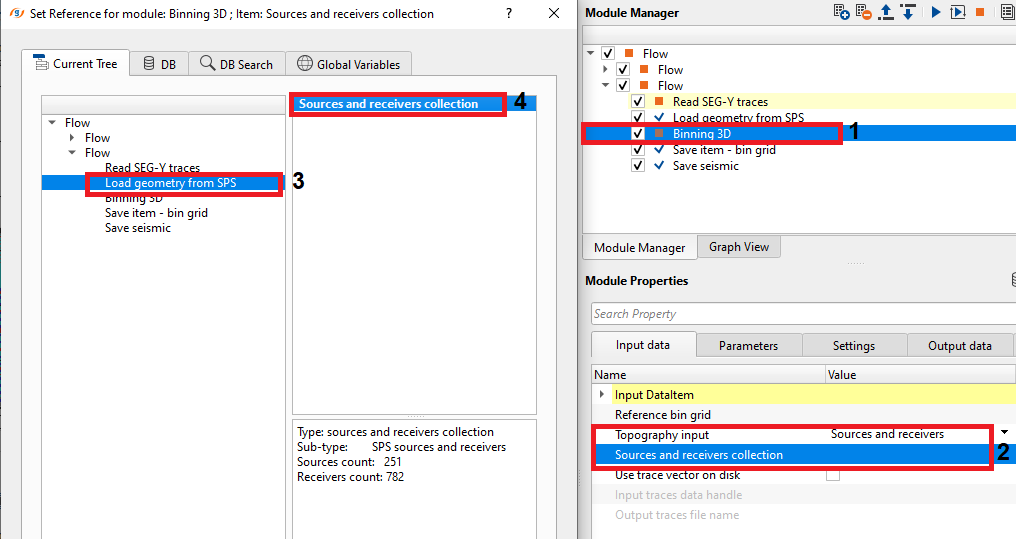
TopographyInput - Sources and receivers collection

The user should provide from where the collection of sources and receivers information should get it from.

Sources and receivers collection

In this case, the user should connect/reference to the source and receiver collection of "Load geometry from SPS" module or any other navigation module.

TopographyInput - External file

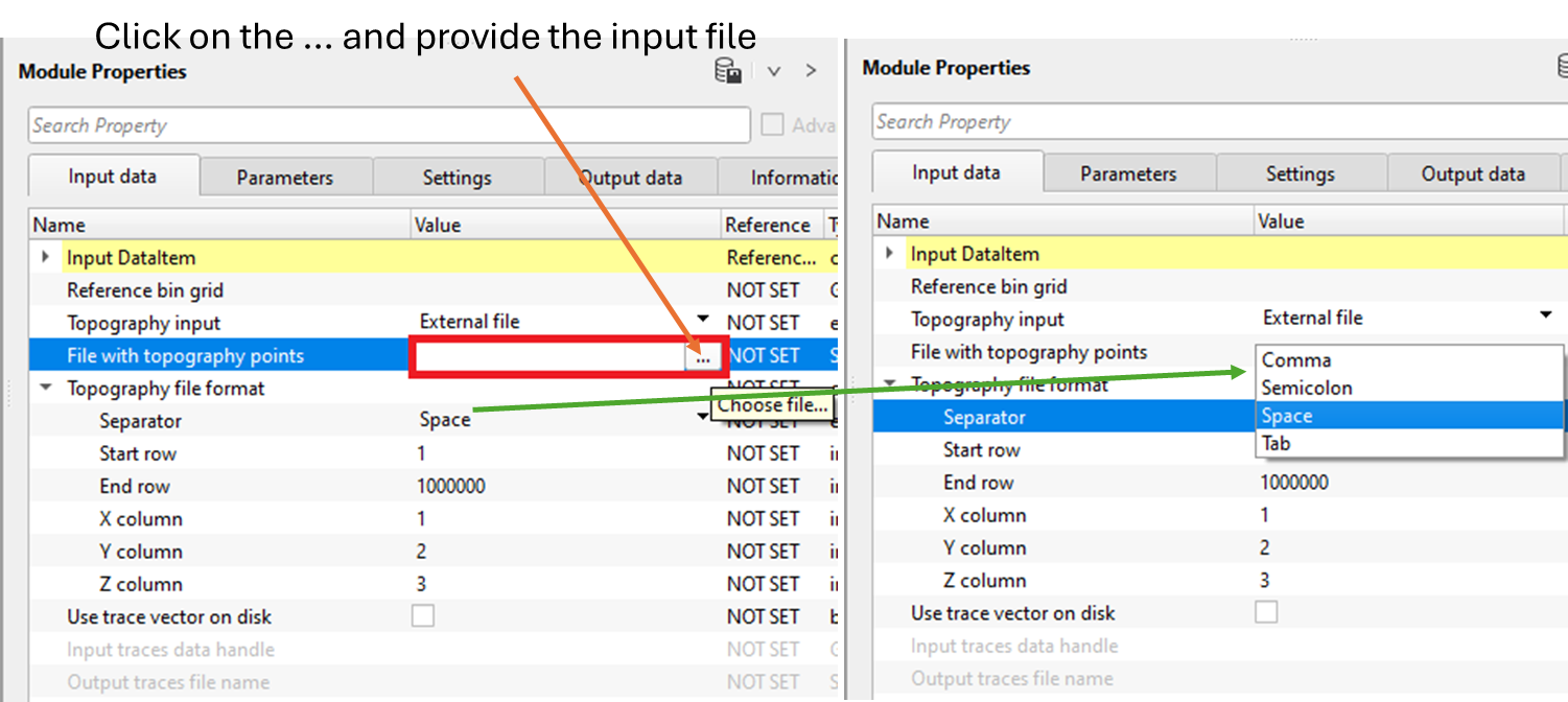
Provide the external file name which consists of the topography information.

File with topography points

Provide the input file path which consists of the topography information.

Topography file format

Select the file format from the drop down menu.

Separator { Comma, Semicolon, Space, Tab }

By default, Space.

Start row

Specify the starting row of the external input file.

End row

Specify the ending row of the external input file.

X column

Specify the X co-ordinates column number.

Y column

Specify the Y co-ordinates column number.

Z column

Specify the Depth column number.

TopographyInput - External map

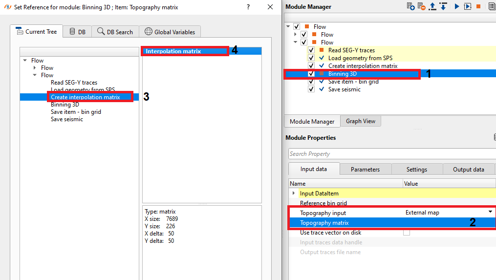
This option provides to input any external maps which has topography information.

Topography matrix

This should be referenced to the Topography index. Here we are referencing into Interpolation matrix of "Create interpolation matrix" module. Inside the create interpolation matrix, we've provided source and receiver elevations to create the topography matrix.

TopographyInput - Marine data

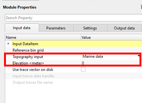
This option is for the offshore data where we don't deal with the elevations of the source and receivers but the depths.

Elevation

By default, 0. In this case, the topography elevation should be Zero (0) which is nothing but the Mean Sea Level (MSL) for any topography reference.

Use trace vector on disk

This option is useful when the input data is too big. Check this option to activate the trace vector on disk.

UseTraceVectorOnDisk - false

By default, False (unchecked).

UseTraceVectorOnDisk - true

If this is true, the user should connect/reference the input traces data handle.

Input traces data handle

Connect/reference to Output traces data handle of Open seismic traces module.

Output traces file name

Use trace vector on disk is used when we read big size of seismic data for faster execution. In this case, instead of using "Read seismic traces" module, we use "Open seismic traces" module. This module is useful for reading internal data formats only. When using Open seismic data only we can use this option.

Parameters

Use only live traces

By default, TRUE (Checked). While doing the binning, it will consider all the live traces (trace_type as 1). Any other trace types will be discarded if this option is checked.

Grid definition

This is where all the grid information should be provided.

Shift grid to center of bin

By default, TRUE (Checked). This will shift all the bin positions to the center of the grid.

Grid starting point - X coord

Provide the grid starting point of the x-coordinate

Grid starting point - Y coord

Provide the grid starting point of the y-coordinate

Inline azimuth

Provide the inline azimuth angle.

First inline number

It's up to the user's choice. Specify the 1st inline number to be considered while doing the binning.

First crossline number

Specify the 1st Xline number.

InLine distance

By default, 10000. This is automatically calculated based on the grid starting point coordinates.

Crossline distance

By default, 10000. This is also automatically calculated. This is the length of the crossline.

Angle between inline and crossline

This should be a right angle i.e. 90 degrees.

Master grid definition

This is where the user provides the 3 corner points of the bin grid.

First corner point - X coordinate

Specify the x-coordinate of the 1st corner point.

First corner point - Y coordinate

Specify the y-coordinate of the 1st corner point.

Inline direction corner point - X coordinate

Specify the x-coordinate corner point along the inline direction

Inline direction corner point - Y coordinate

Specify the y-coordinate corner point along the inline direction

Crossline direction corner point - X coordinate

Specify the x-coordinate corner point along the xline direction

Crossline direction corner point - Y coordinate

Specify the y-coordinate corner point along the xline direction

Number of Inlines to add before corner point 1

Define any additional inlines needs to added before 1st corner point. This will extend the bin grid.

Number of crosslines to add before corner point 1

Define any additional xlines needs to added before 1st corner point. This will extend the bin grid.

Number of Inlines to add after corner point 4

Define any additional inlines needs to added before 4th corner point. This will extend the bin grid.

Number of crosslines to add after corner point 4

Define any additional inlines needs to added before 4th corner point. This will extend the bin grid.

Inline bin spacing

This is the bin grid size. Specify the inline bin spacing.

The inline bin spacing is the distance in meters between adjacent bin centers measured along the inline direction. Default value is 50 m. This value should match the nominal source-receiver midpoint sampling interval along the inline direction in your survey design. For land surveys, this is typically half the shot interval. Smaller bin sizes produce a higher-resolution fold map and better spatial sampling of the wavefield, but increase processing time and data volume. Larger bin sizes improve fold but reduce spatial resolution. The bin spacing is also used to compute the total and calculated cube areas reported in the output statistics.

Crossline bin spacing

This is the bin grid size of the crossline direction.

The crossline bin spacing is the distance in meters between adjacent bin centers measured perpendicular to the inline direction. Default value is 50 m. This value corresponds to the nominal midpoint sampling interval across the receiver spread. In a typical orthogonal land 3D survey, this equals half the receiver line interval. Crossline spacing is usually equal to the inline spacing, but for wide-azimuth or narrow-azimuth acquisitions it may differ. The crossline spacing, together with the inline spacing, determines the spatial extent of each bin cell and is used directly in computing the fold map and areal statistics.

GUI parameters

This parameter section is used to set the parameters for visualization purpose.

IL/XL GUI marks grid step

Specify the step size of Inline and Xline markings. Default, 100. It will print/mark the every 100th Inline and Xline

Minimum fold for areal coverage calculation - Minimum fold for calculating full size (square meters) of the area. This information will be displayed on the Information tab along with other grid statistics information

This threshold controls which bins are counted when computing the Calculated cube size output statistic. Only bins whose fold equals or exceeds this value are included in the calculated area (in sq. km). The default value is 0, which counts all bins that received at least one trace. Increasing this threshold — for example to 10 or 20 — filters out poorly sampled edge bins and gives a more representative estimate of the effectively covered survey area. Use this setting to match your survey acceptance criteria: set it to the minimum production fold your processing sequence requires.

Topography parameters

Interpolation method { Triangulation, Abos, Kriging }

Interpolation method - Triangulation

In this interpolation method, it creates network of triangle from a set of data points. One of the commonly used triangulation method for interpolation is Delaunay. It ensures that no data point is inside the circumcircle of any triangle in the mesh. This produces a set of non-overlapping triangles where every point lies on the edge of one of these triangles. A linear interpolation will take place where the value at any point inside a triangle is estimated by taking a weighted average of the three vertices of the triangle.

Elevation type { Sources and receivers, Receivers, Sources }

select the elevations information from the drop down menu.

Sources and receivers

it will take the source and receiver elevations for the interpolation.

Receivers

receiver elevations will be considered for the interpolation and later for the creation of topography maps.

Sources

source elevations will be considered for the interpolation.  

Smoothing distance

Specify the smoothing distance used the interpolation.

Interpolation method - Abos

Artificial Bounded Object Structure or ABOS is a specialized interpolation method where it uses an artificial bounded structure like network of polygons to model and interpolate the elevations information to create the topography map.

Elevation type { Sources and receivers, Receivers, Sources }

select the elevations information from the drop down menu.

Sources and receivers

it will take the source and receiver elevations for the interpolation.

Receivers

receiver elevations will be considered for the interpolation and later for the creation of topography maps.

Sources

source elevations will be considered for the interpolation.  

Smoothing distance

Specify the smoothing distance used the interpolation.

Interpolation method - Kriging

Kriging is a statistical interpolation method based on the assumption that the spatial data points are correlated. It creates an optimal surface that minimizes prediction errors by considering both the distance between data points and their spatial correlation.

Elevation type { Sources and receivers, Receivers, Sources }

select the elevations information from the drop down menu.

Sources and receivers

it will take the source and receiver elevations for the interpolation.

Receivers

receiver elevations will be considered for the interpolation and later for the creation of topography maps.

Sources

source elevations will be considered for the interpolation.  

Smoothing distance

Specify the smoothing distance used the interpolation.

Kriging covariance type { Exponential, Spherical, Gaussian }

Choose the covariance type from the drop down menu.

Exponential

This can be used where the subsurface properties change abruptly over small distances.

Spherical

The Spherical model is useful when the data exhibits a more gradual spatial correlation up to a certain range and then behaves independently beyond that range. When subsurface structures have coherent properties within a certain distance but lose coherence at greater distances.

Gaussian

The Gaussian model is often applied in cases where there is a long-range, gradual spatial dependence between data points. It’s suitable for data where the spatial dependence does not drop off abruptly, such as when seismic properties gradually change over larger distances or in homogenous subsurface areas.

Kriging range

If two data points are closer than the kriging range, they are considered spatially correlated and will influence each other's estimated values. If the distance is greater than the range, their influence on each other will be ignored. If the distance between two data points is more than 500 then it assumes that the data beyond that limit there is no correlation.

Kriging number of points -

Total number of data points used to estimate/interpolate the unknown point/sample. The more the kriging points the better result however the computation time also increase with this.

Write bin elevation headers from { Smoothed map, Unsmoothed map }

This parameter allows the user to choose which elevation map information is used to update the CMP/Bin elevation information.

This choice determines the elevation value written to each bin trace header after binning. Choose Smoothed map (default) when the bin elevation headers will be used as a floating datum for statics corrections, such as in MultiFocusing or surface-consistent statics workflows — the smoothed topography provides a stable datum free from short-wavelength noise. Choose Unsmoothed map when you need the original field elevation at each bin center, for example when archiving raw geometry or when comparing the binned topography against external elevation data for QC purposes.

Smoothed map - Used as a floating datum and the elevations are smoothed by a smoothing factor provided by the user

Unsmoothed map - These are the field/original elevations and there is no smoothing applied.

Rose Diagram

This is a polar plot which displays the directional data i.e. azimuthal information in the survey area.

The rose diagram parameters control the resolution and extent of the offset-azimuth QC display produced after binning. This display shows how trace coverage is distributed in offset-azimuth space, which is essential for assessing the azimuthal balance of a wide-azimuth survey and identifying acquisition gaps or biases. Finer increments (smaller azimuth and offset values) produce a higher-resolution rose diagram but require more memory and computation time. The rose diagram is available as a Vista view after execution.

Offset increment

Define the offset increment value in meters.

Azimuth increment

Define the azimuth increment value in degrees.

Maximum offset

Specify maximum offset to be considered in the rose diagram generation.

Trace selection azimuth index (-1 all indexes)

By default, -1 which means considers all the traces within the survey area.

Advanced

This section contains a parameter that controls an internal safeguard for the bin grid construction. It is not normally necessary to change this setting for well-conditioned surveys, but it may need adjustment in exceptional cases where coordinate ranges are unusually large or where coordinate values are close to zero.

Limit for distance of bingrid

This parameter limits the distance of the bin grid along the X and Y axis. By default, 100,000. If the bin grid X and Y co-ordinates have Zero then it will take a lot of time to build the grid. To avoid that, we limit the distance of the bin grid.

Performance

These options control what is computed and displayed during and after execution.

Disabling computationally expensive options in this group can significantly reduce the total execution time for very large datasets. For example, if you are doing a quick trial binning to preview the grid layout only, you may disable QC attribute map generation and SRB map filling to obtain results faster. Re-enable these options for a final production run where the fold map, offset maps, centroid misfit maps, and source/receiver/bin relationship data are required for QC.

Calc QC attributes, maps

By default, TRUE. If checked, this will calculate and generate the QC attribute maps.

Update MP vista item

This will update the MidPoint vista items.

Update CMP vista item

This will update the Common Mid Point vista items.

UNSAFE

If this parameter is TRUE (Checked), it doesn't create the updated output trace headers. This is used when there is a limitation of RAM usage.

Fill SRB maps for output headers

This option is necessary to show the commutations for the Source/Receiver/CMP on clicking on the location map.

Settings

Auto-connection

By default, TRUE (Checked).

Number of threads

One less than total no of nodes/threads to execute a job in multi-thread mode.

Skip

By default, FALSE(Unchecked). This option helps to bypass the module from the workflow.

Output data

Output DataItem

Output trace headers

This will output updated trace headers which consists of the bin information, inline, crosslines etc.

Output bin grid

Output bin grid can be used for later purpose.

Information

Number of inlines

Total number of Inlines of the survey area

Number of crosslines

Total number of Crosslines of the survey area

Number of input traces

Total number of input traces before binning

Number of traces used

Total number of traces participated in the binning

Number of traces outside the grid - removed

Total number of traces falling outside the bin grid.

Total cube size <sqkm>

This is the total cube size which includes all the additional inline/crosslines included within the bin grid parameters.

Calculated cube size <sqkm>

This is the actual cube size of the survey area where the total number of traces considered in the binning process.

Area of shots

 This information shows the area covered by shots. This is updated by clicking on the update Statistics option in the action items menu.

Number of shots

Total number of shots in the survey area

Shot density <# per sqkm>

Number of shots per sq.km

Area of receivers

This information shows the area covered by receivers. This is updated by clicking on the update Statistics option in the action items menu.

Number of receivers

Total number of receivers in the survey area.

Receiver density <# per sqkm>

Number of receivers per sq.km

Examples

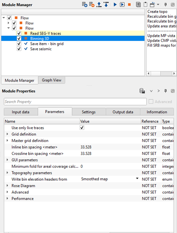
In this example, we are using Teapot Dome 3D example dataset.Here,we are reading the input seismic data by "Read SEG-Y traces". module. For this input data, we've all the geometry information in the trace headers. So we don't have to do any geometry assignment.

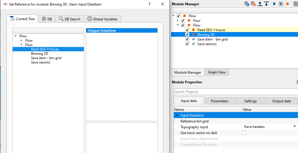
We've connected/referenced the Input DataItem to Output DataItem of "Read SEG-Y traces" module.

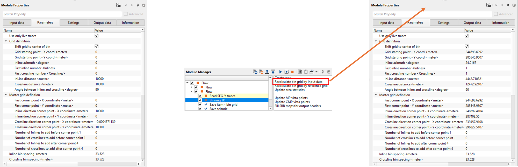
Provide the required bin grid parameters information. In case the user doesn't have the bin grid information, we've an option to get all the bin grid information from the input trace headers by clicking on "Recalculate bin grid information by input data".

Binning 3D generates various QC displays which we call it as Vista items. Generate all the Vista items by right click on Binning 3D -> Vista Groups -> All Groups -> In new window. It will display bunch of QC displays as shown below.

Actions

Custom actions - These are some of the action items that are available to the user to perform various tasks.

Create topo

This will create topography map

Recalculate bin grid by input data

If there are no bin grid information is available, then the user can select this option and it will recalculate the bin grid i.e. bin grid starting and ending points, master grid information etc.

Recalculate bin grid by reference grid

In case the user specified the reference grid in the Input data Tab, based on the reference bin grid, it will recalculate the bin grid information for the input trace headers.

Update area statistics

This will update area statistics in the information tab if the user made any changes to the bin grid information like adding additional inline/crosslines, changing the starting and/or ending bin grid position etc.

----------------------------

Update MP vista points

This will allow the user to update the Mid Points map. Be careful with this option, it will consume lot of time to create the map.

Update CMP vista points

This will update the CMP X&Y Co-ordinates on the map.

Fill SRB maps for output headers

This option is necessary to show the commutations for the Source/Receiver/CMP on clicking on the location map.

Video lesson

YouTube video lesson, click here to open [VIDEO IN PROCESS...]

Related articles

Yilmaz. O., 1987, Seismic data processing: Society of Exploration Geophysicist

* * *   If you have any questions, please send an e-mail to: support@geomage.com  * * *

References

Vermeer, G. J. O., 2002, 3-D Seismic Survey Design: Society of Exploration Geophysicists.