Removing incoherent noise from repetitive shots iteratively
![]()
![]()
What Is Deblending?
Deblending is the process of separating overlapping seismic records that were acquired using simultaneous sources. When two or more sources fire at nearly the same time, their seismic wavefields overlap (“blend”). Deblending removes this interference and recovers individual shot gathers.
Why Do We Perform Simultaneous Source Acquisition?
Simultaneous source acquisition (also called blended acquisition) is used to:
Increase acquisition speed
•Multiple sources fire without waiting for each other → MUCH faster surveys.
Reduce operational cost
•Fewer idle times
•Less fuel + vessel time (marine)
•Faster crew productivity (land)
Increase fold per day
•More shots recorded per unit time.
Improve sampling
•More dense shot coverage at lower cost.
Enable exploration in time-restricted zones
•Weather windows
•Fishing zones
•Military restricted periods
Why Is Deblending Necessary?
Because simultaneous firing creates overlapping wavefields, which causes:
•Cross-talk noise
•Interference
•Incorrect amplitudes
•Difficulty in picking first breaks
•Poor velocity analysis
•Poor imaging
To use blended data in normal seismic processing, we must separate each source’s contribution.
What Is Iterative Deblending & how it works?
Iterative deblending is the most widely used technique.
Deblending relies on two facts:
1.Signal is coherent
(events follow moveout, look like reflections)
2.Interference noise is incoherent
(random-looking because the sources fire at varied time dithers)
So we use an iterative loop:
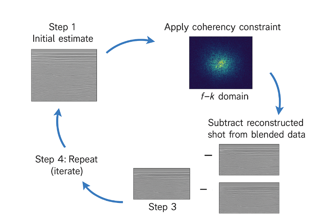
Iterative Deblending Workflow
Step 1 — Initial Estimate
Start by assigning blended data roughly to each source (simple split or a rough filter).
Step 2 — Apply a Coherency Constraint
Reflection energy is coherent in:
•f–k domain
•Radon domain
•Curvelet domain
Noise is not.
We keep coherent energy → throw away incoherent noise.
Step 3 — Subtract Reconstructed Shot from Blended Data
This removes interference progressively.
Step 4 — Repeat (Iterate)
Each iteration:
•Improves signal
•Reduces cross-talk
•Enhances reconstruction
After ~30–40 iterations, sources are well separated.
Shot Times in Simultaneous Source Acquisition
In simultaneous acquisition, multiple sources fire without waiting for previous shots. But to make deblending possible, the shot times are randomized (a technique called dithering).
Types of dithering:
1.Random time dithering (most common)
2.Linear dithering
3.Variable time delays
4.Orchestrated firing patterns
These shot times create incoherent interference, which is much easier to separate from coherent reflections.
How Shot Times Are Created / Recorded
Shot times originate from the acquisition system and GPS clock.
Step 1: Synchronization
All sources and recording systems are synchronized to:
•GPS
•Rubidium clocks
•Precision timing units
This ensures microsecond accuracy.
Step 2: Shot firing command
The acquisition controller sends a firing signal to the source:
•Airgun controller (marine)
•Vibroseis controller (land)
•Explosive detonation unit (legacy)
Step 3: Exact firing time stamp recorded
The shot time is written into:
•Shot header files
•Observer logs
•SPS source files
•Navigation files
•SEG-D / SEG-B / SEG-Y headers
Step 4: Stored per-trace
Each trace stores:
•Source time
•Time since shot start
•Source sequence number
Role of Shot Times in Deblending
Deblending relies on the fact that:
Different sources fire at different (random) times → so their interference appears incoherent.
Using shot times, the algorithm builds the blended source matrix
Deblending works by reversing this mixing.
Shot times define:
•How much overlap occurs
•How interference patterns appear
•How coherent energy is separated
Without shot times:
•Deblending becomes blind
•Nearly impossible to separate shots correctly
Shot Times in Marine vs Land
Marine (airguns)
•Very accurate (ms to microsecond)
•Stored in navigation files
•Used for source signature corrections
•Used for deblending
Land vibroseis
•Vibroseis sweep has start times
•Phase and phase-locking depend on accurate timing
•Used for correlation
•Used for deblending in simultaneous source vibroseis
Types of Shot Times Files in Acquisition
The shot times appear in:
•SPS files (UKOOA/SEG-P1)
•RPS (receiver) & SPS (source) files
•Marine navigation logs
•SEG-D headers
•Observer logs
•Field notes for explosive shooting
Each system logs:
•Shot number
•Shot timestamp
•Source ID
•Vessel position
•Delay time / dither
![]()
![]()
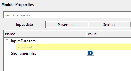
Input DataItem
Input gather - connect/reference to the Output gather for deblending.
Shot times files - provide the shot time files in the tab/space/comma format. Shot time files stores the information about the shot firing time etc.
Each shot time file is a delimited text file (TXT, CSV, or DAT) that records the absolute firing time and source identity for every shot in the blended acquisition. The module reads one or more such files and builds an internal lookup table that maps each source (identified by source line and shot point number) to its precise firing time. This timing information is essential for computing the relative time shifts between simultaneously fired sources, which drive the blending and deblending operators. You must load at least one valid shot time file before the module can run.
![]()
![]()
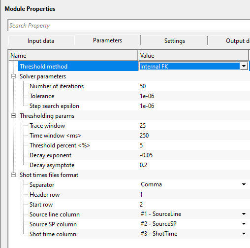
Threshold method { Internal FK, External filter } - threshold method is used to separate/distinguish the coherent and incoherent noise by applying amplitude thresholds in the FK domain or external filter. In case of the External filter, the user should provide the external filter module/procedure under the sub-sequence- External thresholding filter
Threshold method - Internal FK - threshold is applied in the FK domain which results in suppressing the incoherent noise.
Thresholding params - parameters that are determined to suppress the incoherent noise
Trace window - specify the total number of traces to be used for applying threshold. This is also known as spatial window.
The FK thresholding is performed on overlapping patches of data. The trace window defines the lateral size of each patch in number of traces. The default is 25 traces. Larger values capture longer-wavelength coherent events more accurately, but increase computation time. For gathers with dense trace spacing, 20 to 30 traces is typically a good starting range.
Time window - specify the time window/vertical window over which time the FK domain works to suppress the incoherent noise.
This is the vertical (temporal) patch size used in the FK thresholding. It is specified in seconds. The default is 0.25 s (250 ms). Choose a time window large enough to include several reflection cycles at the dominant frequency of your data. If the window is too short, the frequency resolution in the FK domain will be poor and signal may be incorrectly suppressed.
Threshold percent - this parameter determines the strongest/coherent(signal) and weakest/incoherent(noise) events by providing the percentage value.
This is a fractional value between 0 and 1. The module computes the maximum spectral amplitude across all FK patches, then sets the soft-threshold equal to that maximum multiplied by this percentage. The default is 0.05 (5%). A lower value (closer to 0) removes less noise but risks keeping interference; a higher value removes more but may damage weak reflections. Start with the default and adjust if residual noise is visible in the output gather.
Decay exponent - this parameter controls how rapidly the threshold decreases from strong to weak amplitudes.
The threshold level applied in each iteration is scaled by a decay function: (exp(exponent * iteration) + asymptote) / (1 + asymptote). The exponent should be a negative number. The default is -0.05. A more negative value (e.g., -0.1) produces a faster decay, meaning the threshold drops more steeply in the first few iterations and then stabilizes. A value closer to 0 gives a slower, more gradual decay. If deblending converges too quickly and leaves residual noise, try a slower decay (less negative exponent).
Decay asymptote - defines the lower limit of the decay. This parameter determines the minimum attenuation applied to the weakest event/energy.
This sets the floor of the decay function, preventing the threshold from reaching zero at late iterations. The default is 0.2. A higher asymptote means the filter never fully relaxes and continues suppressing weak noise at the end of all iterations. A lower value allows the threshold to become very small, which may be appropriate if you need to recover very weak reflections after most of the interference has been removed.
Solver parameters - this section deals with the solution part of deblending where it controls the iterations, tolerance etc.
Number of iterations - specify the number of iterations required to get better deblending results. The more iterations the better results however more run time.
The default is 50 iterations. Each iteration refines the estimate of the deblended gathers by applying the blending forward operator, computing the residual, and suppressing incoherent noise in the result. More iterations generally produce cleaner separation but add proportionally to processing time. For a quick quality-check run, 10 to 20 iterations may be sufficient; for final production, 50 to 100 iterations are typical. If the solver reaches the specified tolerance before completing all iterations, it stops early automatically.
Tolerance - this parameter defines when the solution to step i.e. lower threshold value where it is achieves the acceptable result. Lower threshold value requires more number of iterations which translates to more run time.
The solver checks convergence at the end of each iteration by comparing the maximum absolute change in the output gather to the maximum amplitude multiplied by this tolerance. The default is 1e-6. When the change falls below this threshold, the solver stops early even if the specified number of iterations has not been reached. In practice, the iteration count usually governs runtime unless a very tight tolerance is set. The default value of 1e-6 is appropriate for most datasets.
Step search epsilon - this is stabilizing parameters that controls the step size to avoid any oscillations or divergence.
Before the main iterative loop begins, the module estimates the optimal step size (learning rate) for the gradient update by computing the largest eigenvalue of the blending operator. This epsilon controls the convergence criterion for that eigenvalue power iteration. The default is 1e-6. This is an advanced parameter: the default value is appropriate for nearly all datasets, and there is rarely a reason to change it.
Shot times files format - this section reads the shot time files provided in the input data.
These parameters tell the module how to parse the shot time file. Before the column selectors (Source line column, Source SP column, Shot time column) become available, you must first load at least one shot time file in the Shot times files input above. The module will then read the header row of that file and populate the column dropdown lists automatically. Make sure that the separator and row numbers match the actual format of your file before executing.
Separator { Comma, Space, Tab } - select the separator type from the drop down menu.
Header row - specify the row position of the header
Start row - specify the starting row of the shot time files from where the actual data starts from
Source line column { None, #1 - SourceLineSourceSPShotTime } - select the source line name from the shot time file
Source SP column { None, #1 - SourceLineSourceSPShotTime } - select the source sp column from the shot time file
Shot time column { None, #1 - SourceLineSourceSPShotTime } - select the shot time column from the shot time file
![]()
![]()
Auto-connection - By default, TRUE(Checked).It will automatically connects to the next module. To avoid auto-connect, the user should uncheck this option.
Bad data values option { Fix, Notify, Continue } - This is applicable whenever there is a bad value or NaN (Not a Number) in the data. By default, Notify. While testing, it is good to opt as Notify option. Once we understand the root cause of it,
the user can either choose the option Fix or Continue. In this way, the job won't stop/fail during the production.
Notify - It will notify the issue if there are any bad values or NaN. This will halt the workflow execution.
Fix - It will fix the bad values and continue executing the workflow.
Continue - This option will continue the execution of the workflow however if there are any bad values or NaN, it won't fix it.
Calculate difference - This option creates the difference display gather between input and output gathers. By default Unchecked. To create a difference, check the option.
Number of threads - One less than total no of nodes/threads to execute a job in multi-thread mode. Limit number of threads on main machine.
Skip - By default, FALSE(Unchecked). This option helps to bypass the module from the workflow.
![]()
![]()
Output DataItem
Output gather - generates the output gather vista. This output gather is deblended gather.
Gather of difference - generates the difference gather before and after deblending. This gather has all the incoherent noise along with the blended shot gathers.
There is no information available for this module so the user can ignore it.
![]()
![]()
In this example workflow, we are reading a synthetic seismic gather with blended shots along with the shot time files.
![]()
![]()
There are no action items available for this module.
![]()
![]()
YouTube video lesson, click here to open [VIDEO IN PROCESS...]
![]()
![]()
Yilmaz. O., 1987, Seismic data processing: Society of Exploration Geophysicist
 * * * If you have any questions, please send an e-mail to: support@geomage.com * * *
![]()