Finding the similarities between two seismic wavelets
![]()
![]()
In seismic data processing, correlation refers to a mathematical measure that helps to understand the relationship between two seismic signals over time. The idea is to find similarities in the seismic data, which can be useful for signal enhancement, noise reduction etc.
There are two types of correlations we can discuss about.
1. Cross-Correlation
Cross-correlation can be used to compare the recorded seismic trace with a known reference signal, such as the theoretical source wavelet. By measuring how well the signals matches/correlate over time, we can identify the time shift i.e. lag that best aligns the signals.
Mathematically, if we define the cross-correlation as two functions, where f(t) and g(t) are two functions separated by a time lag Delta T or Tau. If the cross-correlation function is high it means that both the functions f(t) & g(t) are similar with a time lag.

Cross-correlation helps in
•signal enhancement like signal to noise ratio improvement
•time shift estimations
![]()
2. Auto-Correlation
Auto-correlation is the process of correlating a signal with the signal itself. In seismic data, this technique can be used to identify repeating patterns or periodicity in the data. The auto-correlation function may show a peak at certain intervals, indicating recurring patterns in the seismic activity.
Auto-correlation has its maximum when time lag is zero. It Measures the similarity of a signal to itself over different time lags (useful for identifying periodicity in the data).
![]()
![]()
![]()
Input data
Input gather 1 - Provide the input gather that needs to be considered for correlation
This is the primary seismic dataset. It is the gather whose traces will be correlated against the reference signal. Connect this input to a seismic data reader or to any intermediate processing step that produces the gather you wish to analyze. For auto-correlation mode, only this input is required — the module correlates each trace against itself. If the sample interval of this gather differs from that of Input gather 2, the module automatically resamples both gathers to the finer sample interval before computing the correlation.
Input gather 2 - Provide the second input gather that needs to be considered for correlation
This is the reference gather used in cross-correlation mode. It is not required when Autocorrelation is enabled. Two operating modes are supported depending on the number of traces in this gather:
Single reference trace: If Input gather 2 contains exactly one trace, that trace is used as a common reference signal and correlated against every trace in Input gather 1. This is the classic matched-filter or pilot-trace approach, useful for Vibroseis correlation or wavelet extraction.
Trace-by-trace: If Input gather 2 contains the same number of traces as Input gather 1, each trace pair is correlated independently. Both gathers must have an equal trace count in this mode; otherwise the module will report an error.
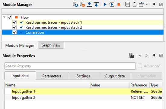
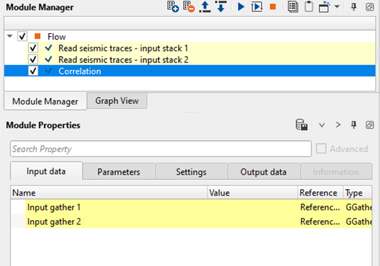
When we use the auto-correlation, we connect/reference to only one input gather. In the above example, we've referenced the input gather 1 to "Read seismic traces - input stack 1". Similarly, if we want to perform the cross-correlation, we'll reference both the input gather 1 and 2.
![]()
![]()
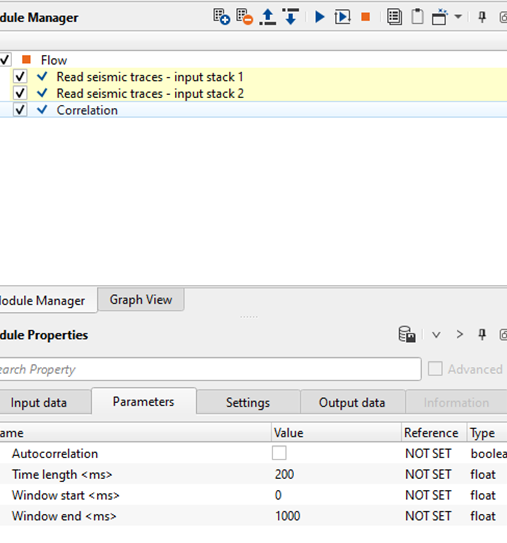
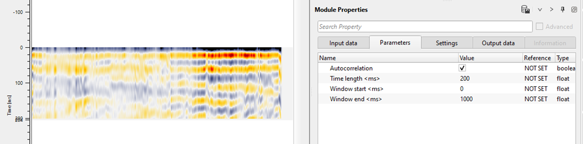
Autocorrelation - By default, Unchecked. If checked this option, it will do the auto-correlation of the same input. When this option is checked, 2nd input gather isn't required.
When Autocorrelation is checked, the module correlates each input trace with itself rather than with a separate reference signal. The second input gather is ignored in this mode. Auto-correlation is particularly useful for analysing the wavelet content of each trace, identifying reverberations or water-bottom multiples, and designing deconvolution operators — the auto-correlation function reveals the periodicity and decay characteristics of unwanted ringing in the data.
Time length - Define the time length that will be used for the correlation. This time length parameter displays the correlation output.
This parameter sets the total duration of the output correlation trace, measured in seconds. The default value is 0.5 s (500 ms). The output correlation function spans from the negative of this value to its positive value, centred on zero lag, so a setting of 0.5 s produces a symmetric output window of 1.0 s total. Increase this value when you need to resolve long-lag features such as deep multiples or far-offset moveout; reduce it to focus on short-lag wavelet details. Set this value smaller than the analysis window length (Window end minus Window start) to avoid edge effects.
Window start - Define the starting time window for the correlation
The start time, in seconds, of the analysis gate over which the correlation is computed. The default value is 0 s. Only the portion of each trace between Window start and Window end is used to compute the correlation function. Restricting the analysis gate to a geologically meaningful interval — for example, the target reflection zone — reduces the influence of noise from other parts of the record and produces a more focused result. Window start must be strictly less than Window end.
Window end - Define the ending time window to perform the correlation
The end time, in seconds, of the analysis gate over which the correlation is computed. The default value is 20 s. Together with Window start, this defines the portion of the input traces used to build the correlation function. If the input data is shorter than the specified window, the module uses the available trace length. Always set Window end to a value greater than Window start; if the two values are equal or reversed, the module will report an error and will not produce output.
![]()
![]()
Skip - By default, No (Unchecked). This option helps to bypass the module from the workflow.
![]()
![]()
Output gather - This module outputs the cross-correlated/auto-correlated gather as an output gather.
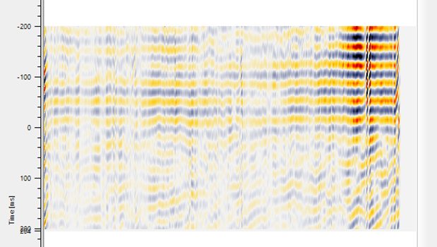
The output is a gather of correlation traces. Each output trace represents the correlation function between the corresponding pair of input traces (or a trace and itself in auto-correlation mode), over the lag range defined by the Time length parameter. The zero-lag sample corresponds to the centre of the output trace, where perfect alignment between the two signals produces the maximum correlation value. The output is displayed by default in the Correlation Vista window in wiggle mode; you can switch to density (colour fill) mode through the View / Show Properties menu of that window. Connect this output to downstream processing modules or to a seismic data writer to save the correlation result for further analysis.
![]()
![]()
In this example, we are reading stack sections. Input gather 1 is a denoise stack and Input gather 2 is also a denoise stack with different processing parameters. We would like to see the results of the cross-correlation and auto-correlation of these stacks sections.
After executing the correlation with the above parameters, we generate the Vista items. We'll get the input 1 & input 2 stack displays and Correlation window display. The default display of the correlation is in wiggle mode. The user can change the wiggle mode to density mode by changing it from the View/show properties of the Correlation window.
For the same stack section, if we want to perform the auto-correlation with the same parameters, we need to turn on/check the Auto-correlation option in the parameters. As mentioned earlier, for auto-correlation, we don't require the 2nd input gather.
Auto-correlation helps in finding out the signal response at the different time lags. It is helpful in designing the deconvolution parameters for any water bottom ringing etc.
![]()
![]()
There are no action items available for this module. So the user can ignore this part.
![]()
![]()
YouTube video lesson, click here to open [VIDEO IN PROCESS...]
![]()
![]()
Yilmaz. O., 1987, Seismic data processing: Society of Exploration Geophysicist
 * * * If you have any questions, please send an e-mail to: support@geomage.com * * *