Adaptively subtracting the noise/multiples from input data
![]()
![]()
Seismic data consists of many unwanted data elements like ground roll, direct arrivals, coherent/incoherent noise, multiples etc.The main objective of any seismic data processing is to attenuate/remove these unwanted noise. During the process, we perform many tasks to attenuate these noise elements depending on the noise nature. Out of the methods, adaptive subtraction is one kind of method where we use extensively to attenuate/remove noise. This method is widely used for multiple attenuation.
How does it work?
Adaptive subtraction works on the principle of subtracting a modeled data set from the input data set in an adaptive fashion. In this, it'll adjust itself based on the characteristics of the data. This is the reason why it is called as Adaptive subtraction.
To preform adaptive subtraction, we need two datasets. One is the original input data with both primary and noise/multiple. On the other hand, we should have a model dataset where the noise/multiple is modeled.
In normal arithmetic subtraction, it will perform a simple subtraction which doesn't consider the phase, amplitude and frequency components. Whereas in the case of adaptive subtraction, it will adjust its characteristics to the input and model data characteristics and dynamically (both in time and space) subtract the unwanted noise/multiple from the input data. For the estimation of the unwanted noise/multiple, it will require a filter often we call it as a Matching filter. This matching filter uses any one of the algorithms like SVD (Singular Value Decompostion), Choleksy Decompostioin, LSQR (Least Square) & FISTA (Fast Iterative Shrinkage Threshold Algorithm) to estimate the unwanted noise/multiple adaptively.
In g-Platform we have two kinds of subtraction types. General Adaptive Subtraction and Arithmetic Subtraction. For SRME, we generally use General Adaptive Subtraction type. For any other subtractions we use the simple Arithmetic subtraction type.
![]()
![]()
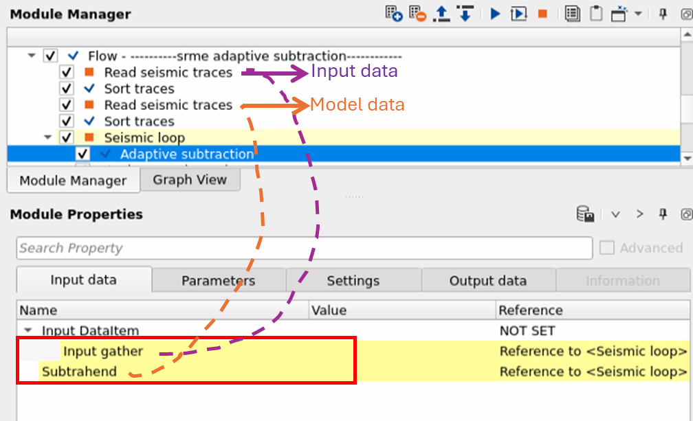
Input DataItem
Input gather - Connect/reference to the input gather which has both primaries and multiples i.e. the original input data
Subtrahend - Connect/reference to the multiple model gather.
![]() For better Multiple attenuation/elimination, it is always advisable to mute the Input data above the water bottom in order to get a better multiple model prediction. Otherwise if we have data above the water bottom, adaptive subtraction treats that as a multiple and try to subtract the primaries from the input data.
For better Multiple attenuation/elimination, it is always advisable to mute the Input data above the water bottom in order to get a better multiple model prediction. Otherwise if we have data above the water bottom, adaptive subtraction treats that as a multiple and try to subtract the primaries from the input data.
![]()
![]()
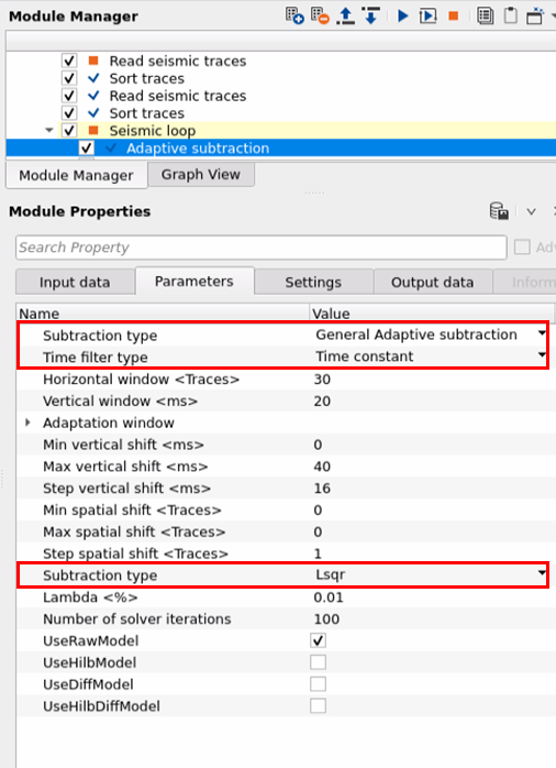
This is the default parameters display of Adaptive subtraction parameters. There are various parameters existing in this module. Depending on the parameter type, the options changes. Some parameters will be disabled and some are enabled.
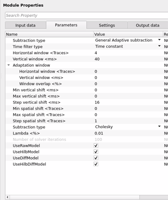
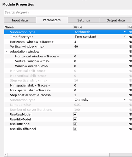
Subtraction type { Arithmetic, General Adaptive subtraction }
Arithmetic - In this option, it will perform a simple arithmetic subtraction like A - B. This can be used for a simple operations however it is less advisable to use in case of multiple attenuation etc.
General Adaptive subtraction - This option perform the adaptive subtraction by designing a matching filter which estimates the unwanted noise/multiple. This method takes into consideration of the input data amplitudes, frequency, phase etc.
Time filter type { Time variant, Time constant, Frequency divided } - These are the filters used to suppress the unwanted noise/multiple from the input data. Depending on the nature of the noise, we use different kinds of time filters. There are 3 types of filters available.
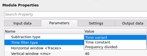
Time variant - Time variant filter is useful whenever there is a continuous change of the noise/multiple characteristics over a period of time. These filters uses information from different time windows and attenuate the noise/multiples. When we select this option, there will be a Time Table parameter option available. Click on the table icon which is marked as a red rectangle. It will pop-up a new window with set of parameters.
Time Table -
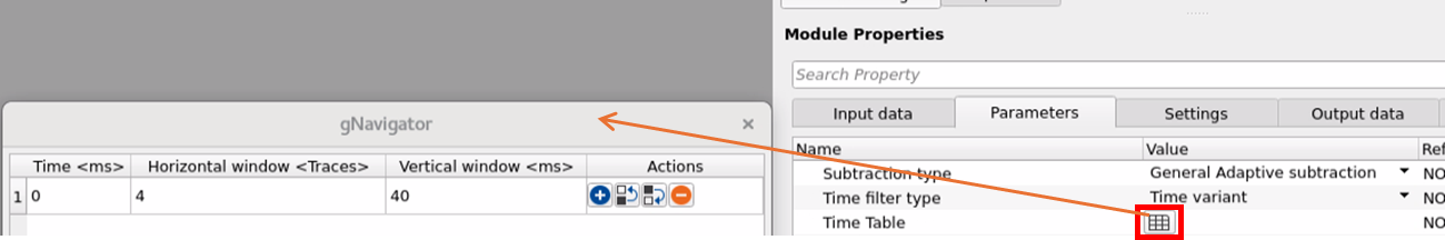
Time - Define the time in milliseconds. Since it is a time variant filter, the user can input different time intervals. At different time intervals, we'll have different horizontal and vertical window parameters. Based on these, the time variant filter adaptively subtract the noise/multiple from the input data using any one of the chosen subtraction type algorithms.
Horizontal window <Traces> - Define number of seismic traces. The set of seismic traces acts as horizontal window.
Vertical window <ms> - Define the time window in milliseconds.
With the combination of both horizontal window and vertical window, it will works like a sliding window with set of seismic traces and in a particular time window. This will process in one window. Once it finishes, it will move on to the next window and it keeps continuing until it finishes all the traces and time sample of the gather.
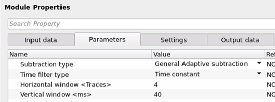
Time constant - This is a constant filter. Irrespective of the data characteristics, it applies a constant filter to the entire seismic data samples. Here, we've horizontal and vertical windows only.
Horizontal window - Provide the number of seismic traces.
Vertical window - Provide the time samples in milliseconds.
Frequency divided - Frequency divided filter divides the seismic data into different frequency bands. These frequency bands are divided using any of the decomposition techniques like Fourier transforms. In this, each frequency band is applied with a filter and combined all of them later. This allows to treat each and every one of the frequency bands differently. In cases where the noise/multiples are having different frequencies, it is really helpful in attenuating the unwanted noise/multiple.
Frequencies table -
When we select the "Time filter type" as Frequency divided, we'll have a + icon symbol at the Frequencies table. Click on it and it will turn the + icon into Table format. Upon clicking the Table icon, it will pop-up a new window. In that window, we've
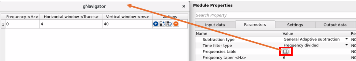
Frequency <Hz> - Provide the frequency values. This is also works like time variant but here we've define the different frequencies and each frequency window will work with the combination of horizontal and vertical windows to estimate the unwanted noise/multiple by using the adaptive subtractive algorithms.
Horizontal window <Traces> - Provide the number of seismic traces.
Vertical window <ms> - Provide the time samples in milliseconds.
Frequency taper - Provide the frequency taper which is required to avoid sharp edges or artifacts at the boundary.
Adaptation window - This parameters defines the portion of seismic data is going through the adaptive subtraction by means of horizontal and vertical window parameters. This adaptation windows determines how the filter adapts to the changes of the local characteristics of the seismic data with respect to horizontally (spatially) and vertically (temporally).
Horizontal window - Total number of seismic traces are participating the adaptation window. Pay attention to number of traces. More number of seismic traces may give good understanding of the spatial variability of the seismic signal however this may not work well in all cases we want finer details. Also, this may increase the computation time.
Vertical window - Provide the time in milliseconds.
Window overlap - This parameter applicable to both horizontal and vertical window parameters. As we know that the adaptation window works in a sliding window pattern, we need to have sufficient traces and time samples as overlap within the sliding window for smoother transition of the adjacent windows. Without a window overlap, we may end up creating noise or artifacts. For example, if the user selects the horizontal window as 5 traces and vertical window as 8ms then within the sliding window, 3 traces will be overlapped from adjacent traces. Similarly, 4ms time overlap is required within two adjacent time samples. So 50% of window overlap will be good for a smoother transition between two adjacent windows.
Min vertical shift - Define the smallest or minimum vertical shift of the data during the filtering process. Usually the seismic data starts from time 0 ms. We can specify this time as a minimum vertical shift. Otherwise, we can define the next available time sample. It will depend on the sample interval of the input data. If the input data is 2ms sample interval then we can put this minimum vertical shift as 2ms. In case it is 4ms then we input this value as 4ms. So, the filtering process will start from 4ms time sample onwards.
Max vertical shift - Specify the maximum vertical shift of the data during the filtering process.
Step vertical shift - Specify the step size of the vertical shift. This step size is usually of sample interval size.
Min spatial shift - Provide the minimum number of traces moving spatially during the filtering process to attenuate the multiples from the input data. This is typically the starting trace of the shot gather. A smaller step size will allows finer details of the data which controls how finely the adaptive filter resolves spatially.
Max spatial shift - Provide the maximum number of traces moving spatially in the filtering process. Too much of maximum spatial shift size will lead to missing important information of the spatial variations of the signal.
Step spatial shift - This is the incremental movement of the filter window across the traces.
Subtraction type { SVD, Cholesky, Lsqr, FISTA } - There are 4 subtraction types are available. The user should select any one of them from the drop down menu and provide the parameters accordingly.
SVD - Singular Vector Decomposition: This method in adaptive subtraction works by decomposing the seismic data matrix into singular vectors and values, then separating the primary signal (high-rank components) from unwanted noise or multiples (low-rank components). By removing or filtering out the low-rank components and reconstructing the data, SVD helps to enhance the primary signal while suppressing multiples or noise.
Cholesky - Cholesky Decomposition: In the Cholesky subtraction method, the primary idea is to use the Cholesky decomposition of the auto-correlation matrix of seismic data to model and subtract multiples from the observed data. The method leverages the correlation structure between seismic traces to isolate and remove these unwanted noise/multiples, thus enhancing the clarity of the primary reflections for further interpretation.
Lsqr - Least Square method is an adaptive filtering technique used to estimate and subtract unwanted signals such as multiples or noise. It involves solving a least squares optimization problem to find the best-fit unwanted signal model, which is then subtracted from the observed data to recover the primary seismic signal. The method is flexible, data-driven, and effective for removing complex unwanted components, but it can be computationally demanding and dependent on the quality of the input data.
FISTA - Fast Iterative Shrinkage Threshold Algorithm is a powerful optimization method used in adaptive subtraction. It helps remove unwanted signals such as multiples or noise by solving sparse recovery problems with an objective function that combines data fidelity and sparsity-promoting regularization (L1 norm). FISTA is faster and more efficient than traditional methods, making it well-suited for handling large seismic datasets while preserving the primary signal and suppressing unwanted noise/multiples.
Lambda - This is a regularization parameters where it is used to control the balance between fitting the data and suppressing the noise/multiple data.
When the estimated multiples are less sensitive to the small variations, a large Lambda value gives more weight to the regularization term which leads to smoother solution. Whereas in the case of lesser Lambda value, the estimated multiples are closely fitted/matched with the input data however this will increase the noise levels also.
Number of solver iterations - Specify the number of times the estimation process to be performed/repeated to achieve the optimum result.
UseRawModel - When the user selects/checks this option, this will uses the raw model which is nothing but the predicted multiple model we supplied as a secondary input to the adaptive subtraction module.
UseHilbModel - When the user chooses this option, it will create the analytical signal which is used to estimate multiples. This model utilizes the Hilbert transformation which focuses on phase and amplitude.
UseDiffModel - This is a Differential operator method. In this method, it uses differential operators to model the changes in the signal, thus helping estimate and remove the multiples that changed rapidly over time and/or space.
UseHilbDiffModel - This is the combination of the Hilbert transformation with Differential operator method. This model is used when the input data is of more complex in nature. Hilbert transformation model work on the phase and amplitudes whereas the Differential operator model works on the changes in the signal to create a robust model to attenuate the multiples from the input.
![]()
![]()
Auto-connection - By default, Yes (Checked)
Bad data values option { Fix, Notify, Continue } - This is applicable whenever there is a bad value or NaN (Not a Number) in the data. By default Notify. While testing, it is good to opt as Notify option. Once we understand the root cause of it, the user can either choose the option Fix or Continue. In this way, the job won't stop/fail during the production.
Calculate difference - This option creates the difference display gather between input and output gathers. By default Unchecked. To create a difference, check the option.
Number of threads - One less than total no of nodes/threads to execute a job in multi-thread mode.
Skip - By default, No (Unchecked). This option helps to bypass the module from the workflow.
![]()
![]()
Output DataItem -
Output gather - The final output from this module is a noise/multiple free output gather.
Gather of difference - This module generates the gather difference between the input and the final output.
![]()
![]()
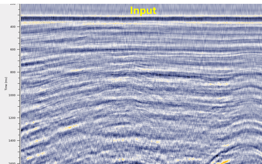
Here is an example workflow to attenuate/remove the multiples by using adaptive subtraction method. In this, we are building the workflow with two "Read seismic traces" modules followed by "Sort traces". We are sorting the data as Channel in Grouping and FFID in Sorting.
As we mentioned earlier, Adaptive subtraction requires two inputs i.e. input data and model data. One input data is connected/referenced to "Read seismic traces" which consists of input data followed by Subtrahend is connected/referenced to another "Read seismic traces" module which is multiple model.
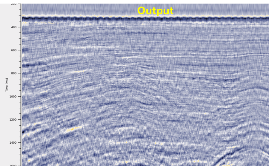
In this workflow, we are using General Adaptive subtraction method with Time Constant and Least Square subtraction type. Here is the result of an adaptive subtraction of an input data and a predicted multiple model as inputs to the Adaptive subtraction module with the following parameters.
![]()
![]()
There are no action items/custom actions are available for this module
![]()
![]()
YouTube video lesson, click here to open [VIDEO IN PROCESS...]
![]()
![]()
Yilmaz. O., 1987, Seismic data processing: Society of Exploration Geophysicist
 * * * If you have any questions, please send an e-mail to: support@geomage.com * * *