Calculating amplitude scaler for geometrical spreading correction
![]()
![]()
Seismic data wave propagation experiences attenuation of seismic energy due to geometrical spreading, absorption, scattering and due to near surface effects. To recover the loss of energy due to these, we compensate the amplitudes by using various amplitude scaling methods. In one of those methods, we've Spherical Divergence Correction which is mostly happens due to the geometrical spreading.
Spherical divergence correction is applied prior to prestack data to compensate the energy loss (amplitude decay) during the wave propagation. As the wavefront expands the energy is spread over a wider area and the amplitude decays with distance from the source. This amplitude decay is called spherical divergence.
To compensate the amplitude decay, we need to test different combinations of spherical divergence corrections viz., T 2, T 2V and T 2V 2with a single velocity function which is typically "Near surface velocity".
If you choose the offset dependent then the equation will be
• SCALAR (t) = (T * V2/ V0) * SQRT (1 + A) , where
• A = (V2– V02) * X2/ (T02* V4), and
• X = offset of this trace,
• T = trace time at offset X,
• T 0= zero-offset time of this event,
• V = stacking velocity, extracted at time T0,
• V 0= surface velocity (extracted from velocity function at time 0), and we assume that T and T0 are related by the NMO equation:
• T2= T02+ (X/V)2
If we choose the offset independent then the equation will be
A = A0(t)+1/
Where A - corrected amplitude at time t
A0 - Observed amplitude at time t
t - two way travel time
![]()
![]()
Input DataItem
Input gather - connect/reference to the input gather. In case the module is inside the seismic loop, the output gather from the previous module will be auto-connected to the spherical divergence correction module.
Vrms model - Input of velocity gather (Vrms=V0 in case this parameter is not provided)
![]()
![]()
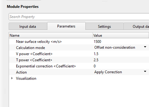
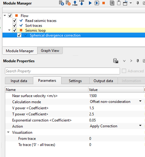
Near surface velocity - Provide near surface velocity or water velocity for marine dataset
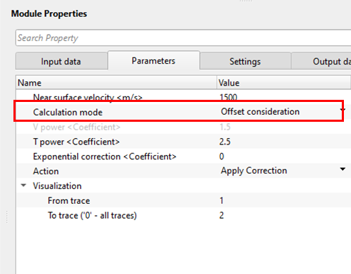
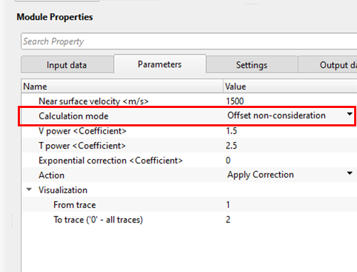
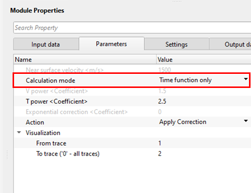
Calculation mode { Offset consideration, Offset non-consideration, Time function only } - We've 3 types of amplitude scalar calculation modes are available.
Offset consideration - When the seismic source like dynamite/vibroseis/air gun fires, the energy penetrates through the sub-surface. During this process the energy is attenuated and dissipated. When the distance(offset) between source and receivers more the energy loss is more. When we consider the offsets in calculating the scalar, then it will consider the t power.
Offset non-consideration - When we consider the offset independent which means, the source-receiver distance (offset) is not a key factor in this calculation. This corrects the amplitude distortion due to the environmental factors and near surface effects. We've consider that the surface wave travel through a constant velocity (near surface velocity) and we've to provide the Time power components.
Time function only - In this case, we are considering the travel time only since the seismic wave propagation happens in homogenous medium.
V power <Coefficient> - If Offset dependent mode is selected this option will be disabled however if the Offset dependent mode is NO then the use should provide the velocity power value like 0.5, 1, 1.5, 2 etc
T power <Coefficient> - Similar to V power, if the Offset dependent mode is selected as NO then the user should provide the T (time) power values like 0.5,1,1.5,2 etc.
Exponential correction <Coefficient> -
Action { Apply Correction, Remove Correction }
Apply Correction - This option lets the user to apply the spherical divergence correction to the data.
Remove Correction - In case the input gather has got the spherical divergence correction already applied, we can remove the earlier applied correction by choosing this option.
Visualization - This parameter is useful to understand the amplitude factor relationship plots. It requires at least 2 traces. It will display the amplitude graph of these two traces. For example, if I've taken From trace is 1 and To trace is 2, it will display the amplitude graph for these two traces only. This is just for visual understanding of how the amplitude graph looks. Spherical divergence correction considers all the traces in the gather irrespective of the visualization parameters.
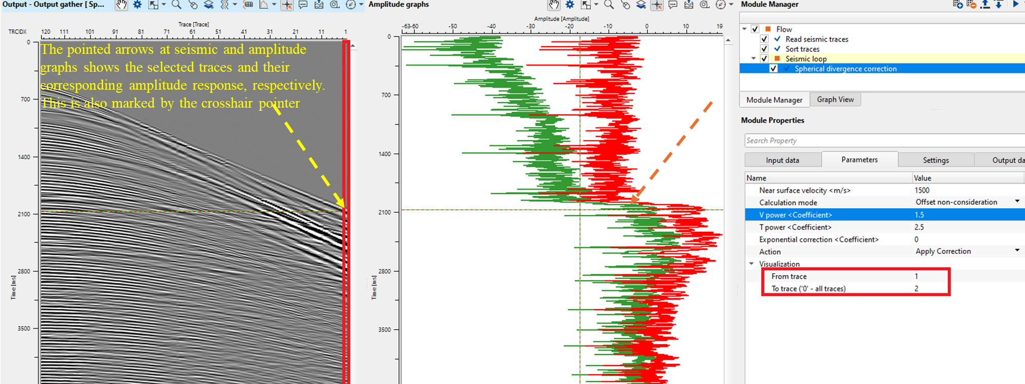
From trace - Provide the starting trace to be considered for the amplitude graph generation. By default, 0 which means it considers all the traces.
To trace ('0' - all traces) - Provide the next trace that needs to be considered for the amplitude generation. By default, 0 which means it considers all the traces.
![]()
![]()
Auto-connection - By default Yes (Checked)
Bad data values option { Fix, Notify, Continue } - This is applicable whenever there is a bad value or NaN (Not a Number) in the data. By default Notify. While testing, it is good to opt as Notify option. Once we understand the root cause of it, the user can either choose the option Fix or Continue. In this way, the job won't stop/fail during the production
Number of threads - One less than total no of nodes/threads to execute a job in multi-thread mode.
Skip - By default, No (Unchecked). This option helps to bypass the module from the workflow.
![]()
![]()
Output DataItem
Output gather - Outputs the spherical divergence corrected output gather
Output scaler factor - Outputs the scaler factor
![]()
![]()
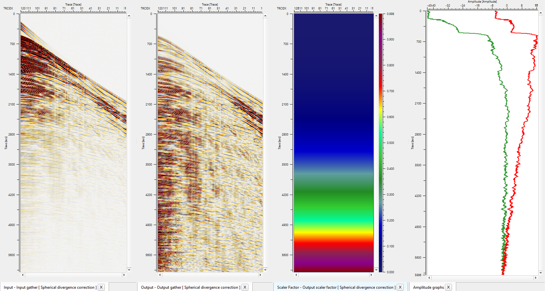
In this workflow, we are reading the geometry assigned gathers by using "Read seismic traces" and sorting the data by FFID and Channel as Grouping and Sorting respectively. Inside the seismic loop, we are adding Spherical divergence correction module.
As per the data requirements, test the appropriate parameters. We'll get 4 QC displays for Spherical divergence as shown below. It'll be Input gather, Output gather after spherical divergence correction, Scale factor and Amplitude Graph.
![]()
![]()
There are no action items are existing for this module so the user can ignore it.
![]()
![]()
YouTube video lesson, click here to open [VIDEO IN PROCESS...]
![]()
![]()
Yilmaz. O., 1987, Seismic data processing: Society of Exploration Geophysicist
 * * * If you have any questions, please send an e-mail to: support@geomage.com * * *