Module performs smoothing of 3D velocity field.
![]()
![]()
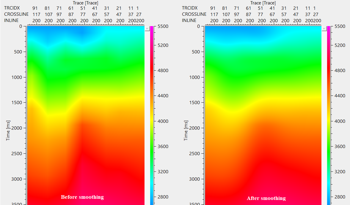
Velocity smoothing in 3D is the process of making a velocity volume (inline × crossline × time/depth) laterally and vertically consistent by removing short-wavelength, non-geological variations while preserving true geological velocity trends.
In 3D, velocities must vary smoothly in both inline and crossline directions, not just along CMPs as in 2D.
1) Large volume of velocity picks - Smoothing enforces global consistency
•3D surveys contain thousands of CMPs
•Manual velocity picking introduces inconsistencies
•Small picking errors propagate across the volume
2) Suppression of acquisition footprint - Smoothing removes non-geological lineations
•3D data often show inline/crossline striping
•These patterns leak into velocity picks
•Un-smooth velocities amplify footprint during migration
3) Geological realism
•Subsurface velocity changes gradually, not abruptly
•Sharp velocity jumps between adjacent CMPs are unrealistic
•Smoothing restores physically meaningful velocity trends
4) Stability of later processing - Smoothing ensures numerical stability
•NMO, stacking, and migration are velocity-sensitive
•Small velocity fluctuations cause large imaging errors
What happens if 3D velocities are NOT smoothed?
In NMO correction
•Events flatten in one inline but not the next
•Residual moveout remains after correction
•Far-offset stretching increases
In stacking
•Poor trace alignment across offsets
•Destructive interference during summation
•Reduced signal-to-noise ratio
In migration
•Migration smiles and frowns appear
•Faults and reflectors lose continuity
•Structural closures become unreliable
In 3D volumes
•Inline/crossline striping
•Velocity footprint dominates the image
•Interpreter confidence reduces
How velocity smoothing is performed in 3D? Velocity smoothing in 3D is applied in three directions:
1) Inline smoothing
•Enforces consistency along survey lines
•Removes line-to-line picking noise
2) Crossline smoothing
•Eliminates striping and footprint
•Ensures lateral continuity between lines
3) Vertical (time/depth) smoothing
•Removes rapid velocity oscillations with time
•Preserves compaction trend
In practice, horizontal smoothing is stronger than vertical smoothing to avoid destroying layering.
Common 3D velocity smoothing methods.
Fast (moving average) smoothing
•Equal weighting inside a window
•Used for quick cleanup
Gaussian smoothing
•Distance-weighted averaging
•Preferred for final velocity volumes
Structure-oriented smoothing
•Follows reflectors
•Preserves faults and dips (advanced Workflows)
Effect of velocity smoothing on NMO
Provides consistent flattening across inlines and crosslines
•Minimizes residual moveout
•Reduces NMO stretch at far offsets
•Produces stable and repeatable stacks
Effect of velocity smoothing on migration
•Stabilizes ray propagation
•Improves focusing of diffracted energy
•Enhances fault definition and reflector continuity
•Reduces migration artefacts caused by velocity noise
What velocity smoothing removes vs preserves
Removes
•Random picking noise
•Inline/crossline acquisition footprint
•Non-physical velocity jumps
Preserves
•Long-wavelength velocity trends
•Structural velocity variations
•Compaction and lithological effects
![]()
![]()
Input DataItem
Use gathers or seismic file { Gather in - gather out, File in - file out } - there are two options for the user to choose from the drop down menu.
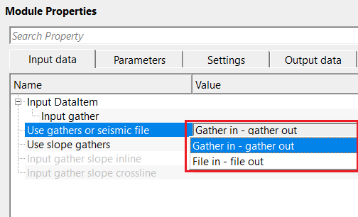
Use gathers or seismic file - Gather in - gather out
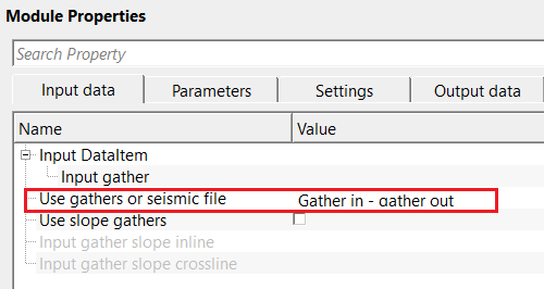
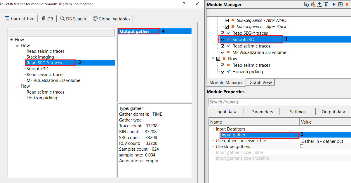
Input gather - connect/reference to the velocity gather that needs to be smoothed.
Use gathers or seismic file - File in - file out
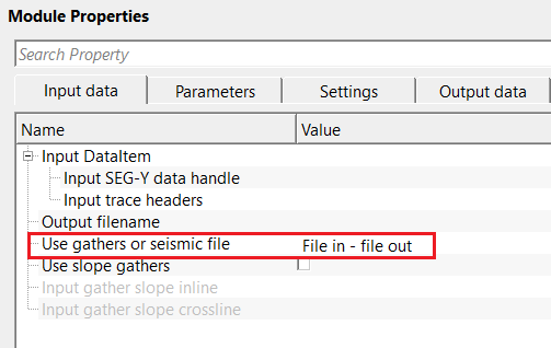
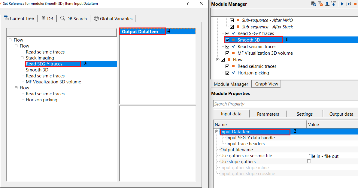
Input SEG-Y data handle - connect/reference to Output SEG-Y data handle.
Input trace headers - connect/reference to the output trace headers.
Output filename - specify the output file name. This generates the smoothed velocity model as an output.
Use slope gathers - by default, FALSE. If checked, the user must provide the inline and crossline slope gathers.
Use slope gathers - true
Input gather slope inline
Input gather slope crossline
![]()
![]()
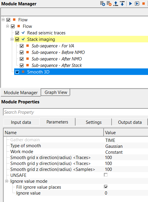
Gather domain { TIME, DEPTH, FREQUENCY } - it automatically detects the input gather domain. By default, TIME. In case the user wants to select the appropriate domain, choose the gather domain from the drop down menu.
Type of smooth { Fast, Gaussian } - there are two types of smoothing options are available. Depending on the requirements of the operation, the user can choose the smoothing type.
Type of smooth - Fast - this is a simple averaging of velocities in a fixed window. Each velocity value is replaced by the mean of nearby samples.
Work mode { Constant, Variant } - select the work mode from the drop down menu.
Work mode - Constant - in this mode, it will be constant values of the horizontal and vertical windows.
Smooth grid x direction(radius) - number of inlines to be considered in the X direction for smoothing
Smooth grid y direction(radius) - number of crosslines to be considered in the Y direction for smoothing
Smooth grid z direction(radius) - number of time/depth samples to be considered for smoothing in the Z direction
Work mode - Variant - this mode works with variable values of both horizontal and vertical windows.
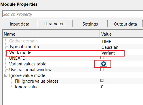
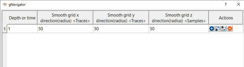
Variant values table - click on the ![]() icon and it will pop-up a new window. Define the respective parameter values in the table.
icon and it will pop-up a new window. Define the respective parameter values in the table.
Use fractional window - by default, FALSE (Unchecked). If checked, it will use
Use dynamic window - by default, FALSE (Unchecked). This option is available when the Type of smoothing is "Fast"
Use dynamic window - true
Max aperture - by default, 5. Maximal number of iterations to find a value that differs from the ignored value.
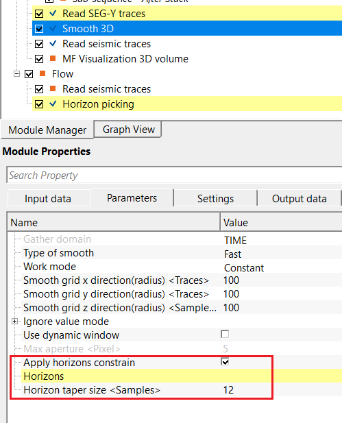
Apply horizons constrain - by default, FALSE (Unchecked). This will give more control to the user to smooth the velocity model based on the horizon.
Apply horizons constrain - true - If the horizon constraint is TRUE, the user should provide the horizon.
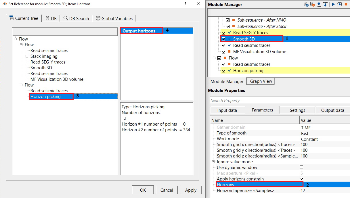
Horizons - connect/reference to the input horizon to control the velocity smoothing.
Horizon taper size - this controls the velocity smoothing. Based on the user specified taper value, it will apply the velocity smoothing below or above the horizon.
Type of smooth - Gaussian - this is a weighted smoothed method by using Gaussian bell shaped function. In this method, nearby samples contribute more than the far samples.
UNSAFE -
Ignore value mode - in this section, the user has the option to ignore some of the velocity values.
Fill ignore value places - by default, FALSE (Unchecked). If TRUE (Checked), replace the sample with smoothed value.
Ignore value - specify the value that should be ignored. Value that will not participate in smoothing algorithm, this value remains as is without changes.
![]()
![]()
Auto-connection - By default, TRUE(Checked).It will automatically connects to the next module. To avoid auto-connect, the user should uncheck this option.
Number of threads - One less than total no of nodes/threads to execute a job in multi-thread mode. Limit number of threads on main machine.
Skip - By default, FALSE(Unchecked). This option helps to bypass the module from the workflow.
![]()
![]()
Output DataItem
Output SEG-Y data handle
Output trace headers
Output gather - outputs the smoothed velocity gather as an output gather.
Calculated inlines count - displays the total number of calculated inlines
Calculated crosslines count - displays the total number of calculated crosslines
![]()
![]()
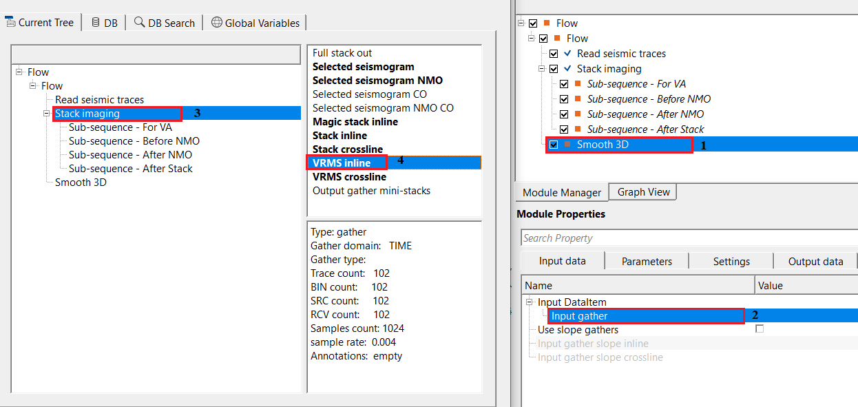
In this example, we've connected/referenced a single inline Vrms velocity as an input to Smooth 3D module. This input is taken from Stack Imaging module.
In case the user wants to smooth the velocity model based on the horizon constraints, then provide the horizon and execute the smooth 3D module. It is necessary to inform to the user that it may take longer time to complete the operation with horizon constraint.
![]()
![]()
There are no action items available for this module.
![]()
![]()
YouTube video lesson, click here to open [VIDEO IN PROCESS...]
![]()
![]()
Yilmaz. O., 1987, Seismic data processing: Society of Exploration Geophysicist
 * * * If you have any questions, please send an e-mail to: support@geomage.com * * *