Removing the seismic wavelet effects by using Wiener Deconvolution
![]()
![]()
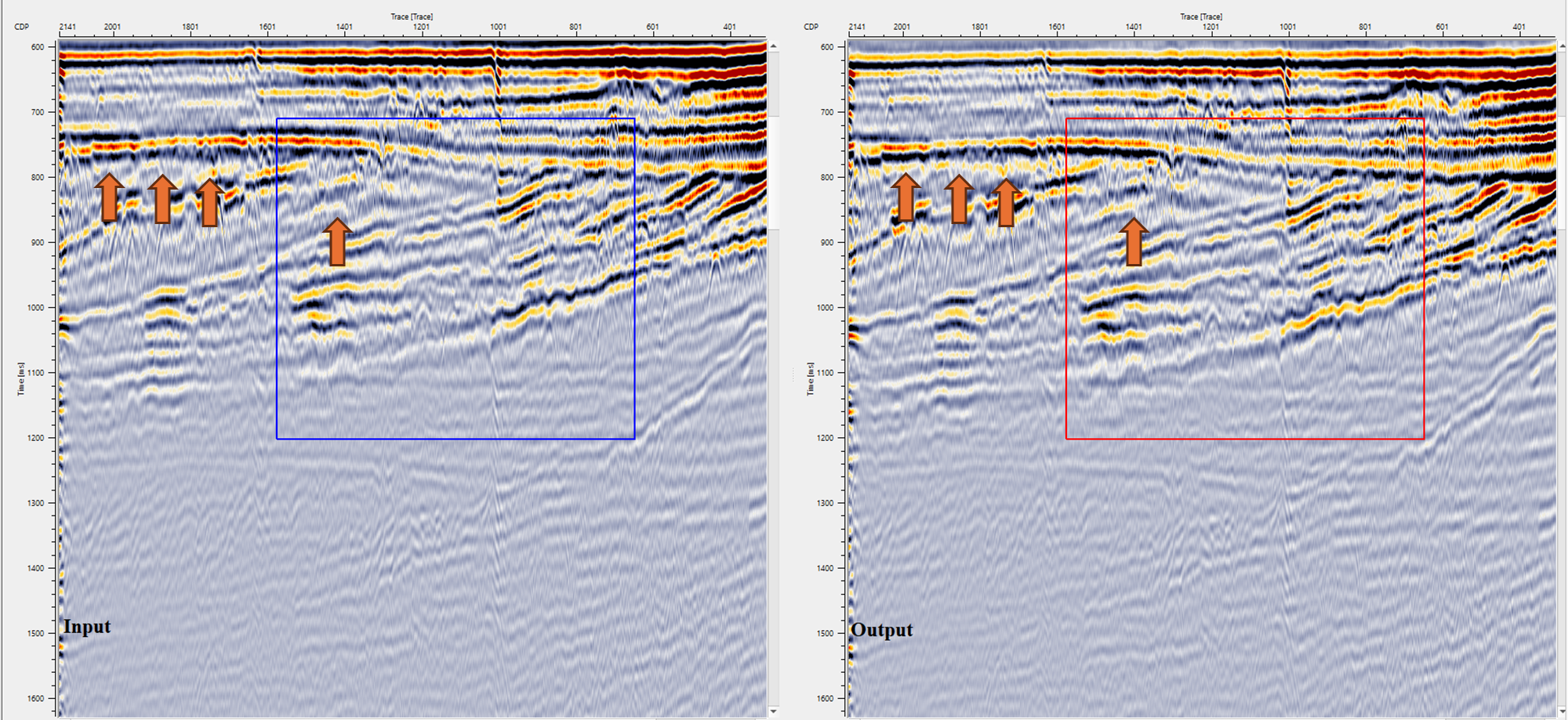
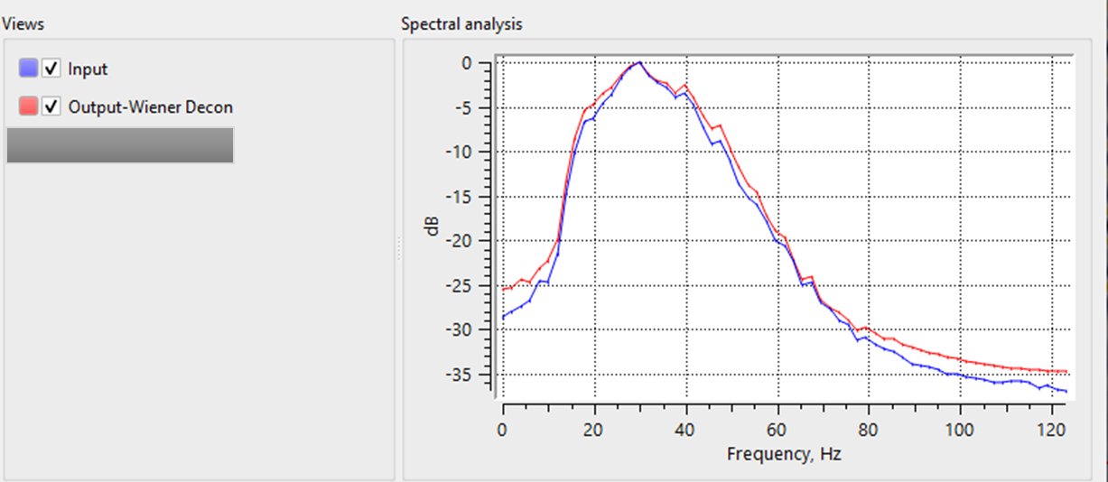
Seismic wavelet undergoes many changes when it first started from the seismic energy source to recorded at the receivers. The wavelet shape changes due to attenuation, dispersion and geological changes like lithology etc. The objective of any deconvolution method is to improve the resolution of the seismic wavelet.
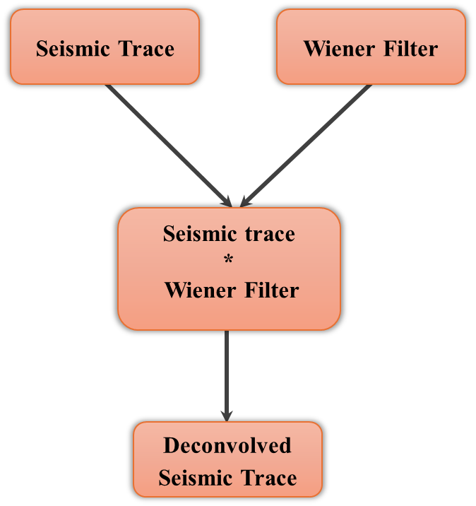
Seismic trace/wavelet is nothing but convolution of source wavelet with reflectivity. This also includes some noise component. As the source wavelet propagates through the sub-surface, it loses the energy and the higher frequencies (travel faster) get attenuated fast compared to the lower frequencies. To restore the reflectivity, we need to design a Wiener filter which minimizes the difference between the estimated reflectivity and original reflectivity.
Where:
•S(t) - seismic trace at time t
•W(t) - seismic wavelet at time t
•R(t) - seismic reflectivity at time t
•N(t) - noise at time t
•* - convolution
Wiener filter was named after Norbert Wiener. Wiener filter tries to minimize the difference between the original seismic signal reflectivity to estimated seismic signal reflectivity. This is called as Mean Square Error or MSE.
Estimated seismic reflectivity is achieved by convolving the seismic trace S(t) with Wiener filter F(t)
When the data is transformed from time domain to frequency domain, convolution becomes multiplication. So the Wiener filter F(f) becomes
Where :
•W(f) - seismic wavelet at frequency f
•S(f) - seismic trace at frequency f
•N(f) - noise at frequency f
•D(f) - density of reflectivity at frequency f
How does Wiener Deconvolution works?
1. Estimate the seismic wavelet S(t) from the input seismic data.
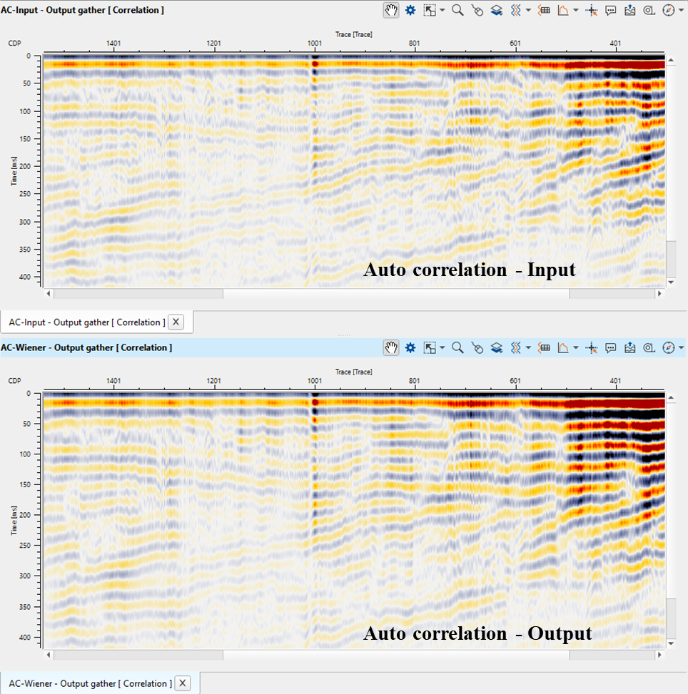
2. Do auto-correlation of seismic wavelet W(t) & seismic trace S(t).
3. Design the Wiener filter W(t) using Wiener - Hopf equation.
4. Convolve the seismic trace S(t) with Wiener filter F(t) to get the estimated reflectivity
Input seismic traces may be zero or minimum phase. According to parameters “Time window” and “Trace window” - traces selected (TT window), which converted into frequency domain (F-X). Then the procedure computes average frequency spectrum for defined TT window and deconvolution operator is computed by the below formula.
Deconvolution operator applying for selected time interval and applying band pass filter to each time interval (for high and low frequency artifacts attenuation). Then all filtered time intervals merged with taper zone. Taper zone equals ¼ of time window interval.
![]()
![]()
Input DataItem
Input gather - connect/reference to the output gather. In case it is inside the Seismic loop module, it will automatically connect/reference to the previous modules output gather.
Connect this item to the seismic gather to be deconvolved. The input can be any pre-stack or post-stack gather in time domain — for example, a CMP gather, a shot gather, or a stacked section. The module processes all traces in the gather simultaneously, using the full lateral extent of the gather to estimate the local average amplitude spectrum within each sliding analysis window. Both zero-phase and minimum-phase input data are supported; set the Min phase parameter accordingly. When placed inside a Seismic Loop, this connector is populated automatically from the previous module's output.
![]()
![]()
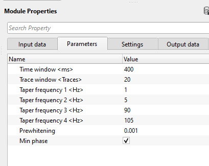
Time window - Time window for Wiener filter calculation. This is also considered as Deconvolution Operator.
The time window (in seconds) defines the length of the sliding analysis gate used to estimate the local average amplitude spectrum from which the Wiener deconvolution operator is derived. The module processes the gather in overlapping time windows and merges the results using a taper zone equal to one quarter of the window length, ensuring smooth transitions between adjacent windows. A shorter window (e.g., 0.2 s) captures rapid spectral changes with depth, which is useful for data with strong Q attenuation; a longer window (e.g., 0.8 s) provides a more statistically stable spectral estimate and is preferable for cleaner, more stationary data. Default: 0.4 s. Minimum: 0.1 s.
Trace window - Trace window for Wiener filter calculation. Specify the number of traces participating in the Wiener filter calculation.
The trace window specifies the half-width (in number of traces) of the 2D sliding analysis patch. The module uses a neighborhood of up to (2 × Trace window + 1) adjacent traces centered on the current trace to compute the average amplitude spectrum for operator design. Including more neighboring traces increases the statistical reliability of the spectral estimate, which is especially helpful for sparse or noisy data. Use smaller values when lateral spectral variation is significant (e.g., in surveys with rapidly changing lithology), and larger values for laterally homogeneous sections. The window is tapered in the trace direction to avoid edge artifacts at patch boundaries. Default: 20 traces. Minimum: 1 trace.
Taper frequency 1 - Frequency taper is applied to each time window/interval to attenuate/filter any artifacts after the application of deconvolution filter. Specify the lower frequency filter taper. Below this value, all frequencies are nullified or considered as zero.
The four taper frequencies (F1, F2, F3, F4) define a trapezoidal band-pass filter that is applied to the Wiener deconvolution operator within each analysis window. This filter suppresses low-frequency and high-frequency artifacts that can be amplified during deconvolution. Taper frequency 1 is the low-cut reject frequency: all energy below this value is zeroed. The filter gain rises linearly from zero at F1 to full pass at F2. Set F1 close to 0 Hz to preserve very low frequencies, or raise it to eliminate ground-roll and very low-frequency noise. Default: 1 Hz.
Taper frequency 2 - specify the filter to be considered. All frequencies above this value are passed.
The low-pass end of the low-frequency taper ramp. The deconvolution operator filter gain rises linearly from zero at F1 to full pass at F2. All frequencies between F2 and F3 are passed at full gain. F2 must be greater than F1. Setting F2 close to F1 produces a steep low-cut slope; widening the gap (e.g., F1=2 Hz, F2=10 Hz) creates a gentler roll-off that better preserves shallow low-frequency energy. Default: 5 Hz.
Taper frequency 3 - specify the higher frequency to be considered. All frequencies inside this value are passed.
The high-pass end of the high-frequency taper ramp. The deconvolution operator filter gain is at full pass between F2 and F3, then declines linearly from F3 down to zero at F4. F3 must be less than F4. Set F3 to match the highest usable signal frequency in your data — typically determined by examining the amplitude spectrum before deconvolution. Raising F3 preserves more high-frequency content but may also preserve high-frequency noise boosted by the deconvolution process. Default: 75 Hz.
Taper frequency 4 - specify the higher frequency value. All frequencies beyond this will be nullified.
The high-cut reject frequency: all energy above this value is zeroed. The filter gain falls linearly from full pass at F3 to zero at F4. Set F4 to a value above the Nyquist-related noise floor, or just above the maximum frequency you wish to preserve. F4 must always be greater than F3. Together, F1–F4 form a trapezoidal (Ormsby-style) bandpass applied to each deconvolution operator window, protecting the output from both low- and high-frequency artifacts introduced by spectral whitening. Default: 80 Hz.
Prewhitening - specify the % while noise added to the data to stabilize the spectrum.
Prewhitening (also called the noise-to-signal ratio or regularization parameter) adds a small stabilizing constant to the denominator of the Wiener filter formula, preventing division by near-zero spectral values at frequency notches. This is the key parameter controlling the trade-off between resolution and noise amplification: a very small value (e.g., 0.0001) produces a sharper, more aggressive deconvolution but can amplify noise at spectral troughs; a larger value (e.g., 0.01 to 0.1) produces a more conservative, noise-tolerant result with less resolution enhancement. The value is expressed as a fraction of the maximum spectral amplitude squared (dimensionless). Start with the default and increase it if the deconvolved output appears noisy or unstable. Default: 0.001 (equivalent to approximately 0.1%).
Min phase - By default, TRUE (Checked). Deconvolution expects the input data in minimum phase (the reason being is that the seismic source generates the energy and the seismic wavelet gets it's maximum energy/peak at the beginning and it gradually decreases. So, it is easier for the deconvolution operator to work on the minimum phase wavelet).
When checked (minimum-phase mode), the module first converts the average amplitude spectrum within each analysis window into a minimum-phase wavelet using spectral factorization (the Kolmogorov method). It then designs the inverse Wiener filter relative to this minimum-phase representation. This mode is the standard choice when the seismic source wavelet is minimum-phase (e.g., dynamite or airgun far-field). When unchecked (zero-phase mode), the module applies a simpler amplitude-only spectral equalization, treating the estimated spectrum as a zero-phase wavelet. Use zero-phase mode when the data has already been phase-corrected or when you want a pure spectral balancing effect without phase rotation. Default: checked (minimum-phase).

![]()
![]()
Auto-connection - By default, TRUE(Checked).It will automatically connects to the next module. To avoid auto-connect, the user should uncheck this option.
Bad data values option { Fix, Notify, Continue } - This is applicable whenever there is a bad value or NaN (Not a Number) in the data. By default, Notify. While testing, it is good to opt as Notify option. Once we understand the root cause of it, the user can either choose the option Fix or Continue. In this way, the job won't stop/fail during the production.
Notify - It will notify the issue if there are any bad values or NaN. This is halt the workflow execution.
Fix - It will fix the bad values and continue executing the workflow.
Continue - This option will continue the execution of the workflow however if there are any bad values or NaN, it won't fix it.
Calculate difference - This option creates the difference display gather between input and output gathers. By default Unchecked. To create a difference, check the option.
Number of threads - One less than total no of nodes/threads to execute a job in multi-thread mode. Limit number of threads on main machine.
Skip - By default, FALSE(Unchecked). This option helps to bypass the module from the workflow.
![]()
![]()
Output DataItem
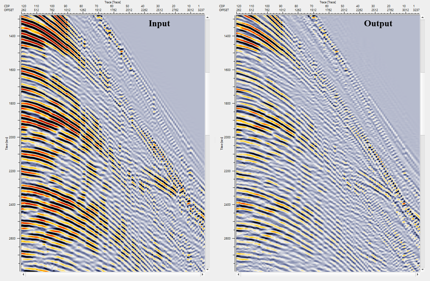
Output gather - generates Wiener filter applied deconvolution output gather.
The deconvolved output gather has the same dimensions (number of traces and samples) as the input. Each trace has been processed by the locally-estimated Wiener inverse filter, resulting in a spectrally balanced, higher-resolution signal. The amplitude is normalized so that the total spectral energy is preserved relative to the input. Connect this output to the next module in your processing workflow for further operations such as stacking, migration, or display.
Gather of difference - generates the difference display gather between input and output gathers.
This optional output contains the sample-by-sample difference between the input and the deconvolved output (input minus output). It is available only when the Calculate difference option is checked in the Settings section. Use this gather as a QC tool to assess what spectral content was removed or altered by the deconvolution — a difference gather that shows coherent reflections indicates over-aggressive deconvolution settings, while a difference gather dominated by incoherent noise indicates a well-balanced result.
There is no information available for this module so the user can ignore it.
![]()
![]()
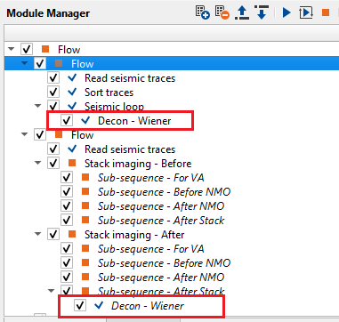
In this example workflow, the user can test different Decon Wiener filter parameters and QC the results.
![]()
![]()
There are no action items available for this module so the user can ignore it.
![]()
![]()
YouTube video lesson, click here to open [VIDEO IN PROCESS...]
![]()
![]()
Yilmaz. O., 1987, Seismic data processing: Society of Exploration Geophysicist
 * * * If you have any questions, please send an e-mail to: support@geomage.com * * *