![]()
![]()
Design a filter to remove the bubble effect and enhance the signal
Bubble is a known issue in the marine seismic data acquisition. When the air gun or any pressure source is used in the marine seismic acquisition as an energy source, it will generate bubbles. These bubbles expand and collapse. Due to this scenario, we can observe a bubble energy near to the water bottom. This can be attenuated by using a debbuling filter.
The main objective of the Debubble is to attenuate the bubble from the source wavelet. Before going to the Debubble, let us discuss about
Why do we need Debubble and what is the procedure and how does it work?
In the marine data acquisition, we use air guns as source. The air gun arrays are designed in such a fashion that we get the desired signal and maximum peak to bubble ratio. Each air gun have different pressure volumes and based on the size of the air gun arrays it will create an impulse. Simultaneously it creates bubbles. Bubbles are created by the expansion and contraction of the air. The period of the bubbles based on the size of the gun array volume. The bigger the size of the gun array volume, more the bubble period. These bubbles appear as low frequency content in the data and we need to attenuate it otherwise they will compromise the resolution of the seismic data. When all the guns (array) fire at the same time, all the peaks will align and add together but the bubbles won’t. By this way we can minimize the bubbles in the data set however there is always some residual bubble left over in the data. To attenuate this we need to design an operator. Designature is the process where we design the operator and attenuate the bubble effect.
How do we design the debubble filter operator?
During the time of acquisition or start of the acquisition, survey companies test various gun array combinations to get the desired source wavelet. They provide the source signature or we can call it as far field source signature. We take this far field source signature and create an operator (wavelet) to get the desired or close to the modeled wavelet. By doing so we attenuate the bubble and we convert the wavelet to minimum phase. Predictive Deconvolution expects the data should be in minimum phase. Deconvolution enhances the signal to noise ratio and attenuates the water reverberations.
There are different ways to get the source signature. If the acquisition company provides the far field signature then it is great, if not then, we can use the near field hydrophone information and design the desired source wavelet. Also, if we have the acquisition report, and the source (air gun) configuration we can design the source wavelet by using some software like Nucleus. There is also another way of doing this. If we have the signature on a paper section we can digitize it and use that also.
There are various kinds of source wavelet to generate. Single source wavelet which is also known as far field signature. Source signature for each individual shot gather. This one is especially available with the modern acquisition. It is called as CMS (Calibrated Marine Signature).
As we discussed earlier, if the user doesn’t have a far field signature then they can generate the wavelet by using the module” Wavelet detection”. To use this, user should read the input shot/receiver/cmp gather or stack section and connect to the Input Dataitem in the Input data tab of the parameters and set the parameters as per the user requirements.
Debubbling of the input data using Far Field Signature
To run Debubble in g-Platform, first we need to read the far field signature by either using the module “Read Wavelet from file” or “Read SEG-Y traces”.
In the following example, we are going to show the option to read the far field signature from the Read SEG-Y traces module and show the result of the debbuling filter.
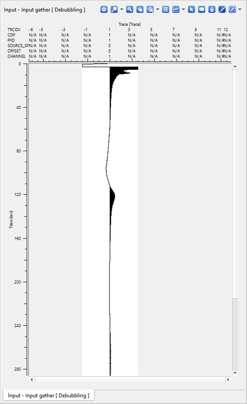
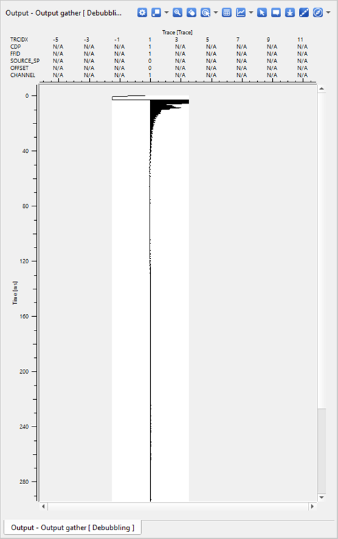
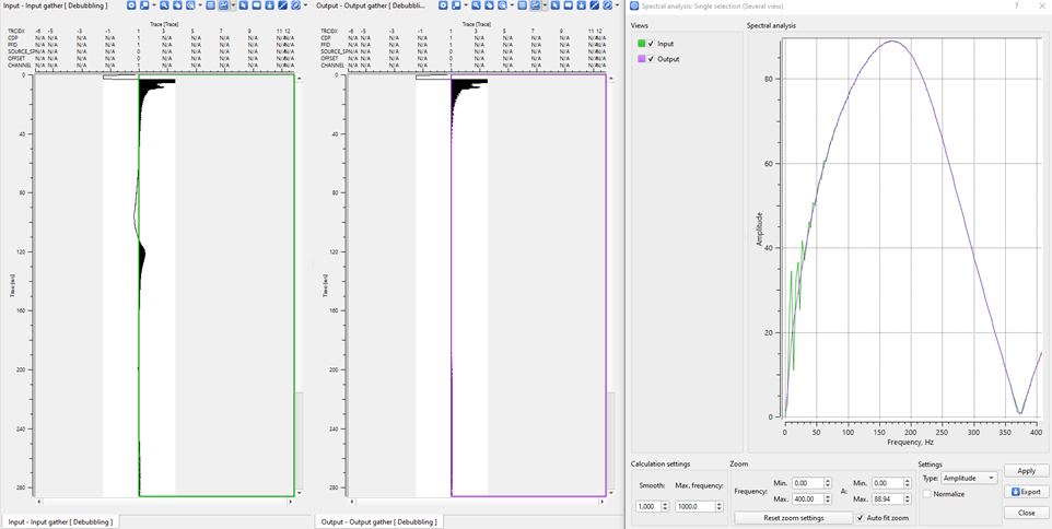
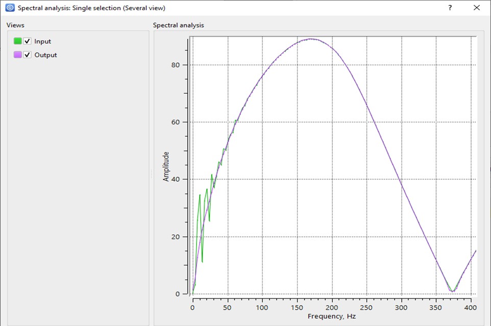
If we look at the spectral analysis of the input and output of the Debubble, we can able to see that the bubble is attenuated successfully
![]()
![]()
In this example, we read the far field signature by Read SEG-Y traces module and connected the same far field signature as an Input wavelet to the Debubbling module.
Input DataItem - Make a reference to Read SEG-Y traces as an Input DataItem of Debubbling module.
Input gather - Make a reference to Output gather of Read SEG-Y traces module (In case, the user doesn't use the Input DataItem as a reference option)
Input wavelet - Connect the input wavelet(in this case far field). In this example, we've referenced it to Read SEG-Y trace module as both input gather and input wavelet are the same.

![]()
![]()
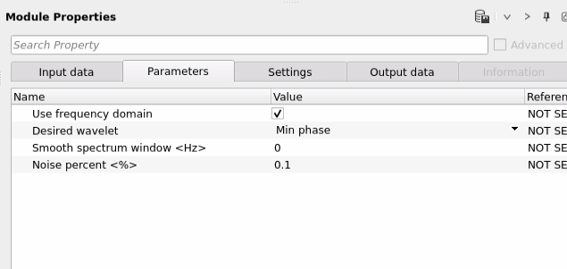
In the parameters, we have selected the desired wavelet as “Min phase”. However if the user wants the desired wavelet as “Zero phase” they can select from the drop down menu of the desired wavelet.
Use frequency domain - By default, it is in the frequency domain. If not, it'll be in time domain.
When enabled (default), the Wiener designature filter is applied in the frequency domain. This is the recommended mode for most datasets: it is computationally efficient and handles long records well. Disable this option to apply the filter as a convolution in the time domain, which may be preferable when working with very short wavelet segments or when frequency-domain edge effects are a concern.
Desired wavelet { Min phase, Zero phase } - Choose from minimum phase or zero phase wavelet as an output desired wavelet from the drop down menu. By default Min phase.
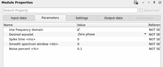
Controls the phase character of the output seismic traces after debubbling. Min phase (default) converts the source wavelet to a minimum-phase equivalent, which is the expected input for predictive deconvolution workflows. Zero phase produces a symmetric wavelet centered at the time defined by the Spike time parameter; this mode is suitable when the data will be interpreted directly without further predictive deconvolution. Select Zero phase and set Spike time to the desired output wavelet peak position in seconds.
Spike time - Define the starting time of the spike. By default, it is Zero (0). If the user specifies the spike time as 50ms then the peak amplitude/spike will be at 50ms of the output.
This parameter is only active when Desired wavelet is set to Zero phase. It sets the time position (in seconds) of the peak of the output zero-phase wavelet, computed via autocorrelation of the debubbled wavelet. The default value of 0 s places the peak at the start of the trace. For standard zero-phase processing, leave this at 0; adjust it only when aligning with a specific target time is required.
Smooth spectrum window - If Zero means there is no smoothing applied to the frequency spectra
Specifies the bandwidth (in Hz) of a running-average smoothing window applied to the amplitude spectrum of the input wavelet before designing the debubble filter. The default value of 0 Hz disables smoothing entirely. Use a non-zero value (e.g., 5–15 Hz) when the input wavelet spectrum is noisy or contains sharp spectral notches that could cause instability in the filter design. Higher values produce a smoother filter at the cost of reduced spectral resolution.
Noise percent - By default, it is 0.1 and it gives the optimum output however, the more the percentage noise we added to the desired wavelet, the less effective of the Debubbling filter. Default value of 0.1 % should be sufficient enough to get the optimum desired wavelet.
A water-level regularization factor added to the denominator of the Wiener inverse filter to prevent division by near-zero spectral values. The value is expressed as a fraction of the peak spectral power (e.g., the default of 0.001 corresponds to 0.1%). Valid range is 0 to 1. Increasing this value stabilizes the filter but reduces the effectiveness of bubble suppression — the filter becomes less aggressive. Decreasing it toward zero makes the filter more powerful but risks amplifying noise at spectral notches. The default of 0.001 (0.1%) is a good starting point; raise it (e.g., to 0.01–0.05) if the output shows ringing or amplified noise.
Taper mode { Auto, Manual } - Controls whether a linear taper is applied to the input wavelet before filter design. Default is Auto (no taper).
In Auto mode (default), the input wavelet is used as-is with no windowing applied. In Manual mode, a linear taper (fade-to-zero ramp) is applied to the wavelet starting at the time defined by Taper start time and decaying to zero over the duration defined by Taper length. Use Manual mode when the wavelet contains late-time noise or ringing (e.g., from reflections recorded on near-field hydrophones) that you want to exclude from the filter design. Selecting Manual reveals the Taper start time and Taper length parameters.
Taper start time - The time (in seconds) at which the linear taper begins to attenuate the input wavelet. Only active when Taper mode is set to Manual. Default is 0 s.
Samples at or before this time are passed through at full amplitude. The taper then ramps linearly from full amplitude at this time down to zero amplitude at the end of the taper window. Set this value to just after the main bubble period in the wavelet — typically a few hundred milliseconds after the first peak — to preserve the meaningful source signal while excluding later noise.
Taper length - The duration (in seconds) over which the linear taper decays from full amplitude to zero. Only active when Taper mode is set to Manual. Default is 0 s.
Increasing the taper length produces a smoother windowing transition and avoids spectral leakage artifacts in the filter design. A taper length of 0 s with Manual mode causes a hard truncation at the start time. In practice, use a taper length of 20–100 ms (0.02–0.1 s) to ensure a smooth fade and stable filter behavior.
Parameters
Use frequency domain - When enabled (default), the Wiener designature filter is applied in the frequency domain, which is computationally efficient and suitable for most datasets. Disable to apply the filter as a time-domain convolution.
Desired wavelet { Min phase, Zero phase } - Selects the phase character of the debubbled output. Min phase (default) converts the source wavelet to a minimum-phase equivalent, required for predictive deconvolution workflows. Zero phase produces a symmetric wavelet centered at the time set by Spike time.
Spike time - Sets the time position (in seconds) of the peak of the zero-phase output wavelet. Only visible when Desired wavelet is set to Zero phase. Default is 0 s (peak at the start of the trace). For example, a value of 0.05 s (50 ms) places the wavelet peak at 50 ms.
Smooth spectrum window - Bandwidth (in Hz) of a running-average smoothing window applied to the wavelet amplitude spectrum before filter design. A value of 0 Hz (default) disables smoothing. Use values of 5–15 Hz when the wavelet spectrum is noisy or contains sharp notches that could destabilize the filter.
Noise percent - A water-level regularization factor (expressed as a fraction of peak spectral power) added to the denominator of the Wiener inverse filter to prevent division by near-zero values. The default of 0.001 (equivalent to 0.1%) balances filter effectiveness against noise amplification. Valid range is 0–1. Increase this value (e.g., to 0.01–0.05) if the output shows ringing or noise amplification; decrease it if bubble suppression is insufficient.
Taper mode { Auto, Manual } - In Auto mode (default), the input wavelet is used without any windowing. In Manual mode, a linear fade-to-zero taper is applied to exclude late-time noise from the wavelet before filter design. Selecting Manual reveals the Taper start time and Taper length parameters.
Taper start time - The time (in seconds) after which the linear taper begins to attenuate the wavelet. Samples at or before this time are passed through at full amplitude. Only visible when Taper mode is Manual. Default is 0 s. Set this to just after the last meaningful bubble oscillation in the wavelet signature.
Taper length - The duration (in seconds) over which the taper decays linearly from full amplitude to zero. Only visible when Taper mode is Manual. Default is 0 s (hard truncation). Use a value of 0.02–0.1 s (20–100 ms) for a smooth transition that avoids spectral leakage artifacts in the filter design.
Creating the wavelet from the input data
In case the far field signature is not available, we still can generate the input wavelet from the input data itself. Here is a detailed outline of the procedure.
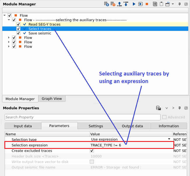
1.Read SEGY data of the all individual sail lines of the entire survey (in case of 3D) using "Read SEG-Y traces". Please make sure to select "All traces" at Load dead traces parameter option in the "Read SEG-Y traces" module. This will consider all the traces including the auxiliary traces.
2.Select the auxiliary traces by using "Select traces" module. Define the Trace Type as per the auxiliary trace id.
3.Save the selected auxiliary traces as an output by "Save seismic" module.
In the next step,
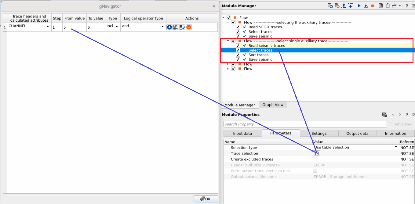
1.Read the previously saved auxiliary traces by using "Read seismic traces" module.
2.Select any particular auxiliary channel. In this example, we've selected channel number 5 by using "Select traces" module.
3.Sort the data by FFID (Optional) by using "Sort traces" module.
4.Save the output (optional) by using "Save seismic" module.
In the final step,
1.Read the previously saved single auxiliary trace (channel number 5) by using "Read seismic traces" module.
2.Sort the data in FFID Grouping by using "Sort traces" module.
3.Reference the input data item and sort traces of the respective modules to "Seismic loop" module.
4.Add "Band-pass filter" (optional) inside the Seismic loop if necessary based on the input data wavelet.
5.Add "Set gather" module. This will combine all the individual auxiliary traces into a single file.
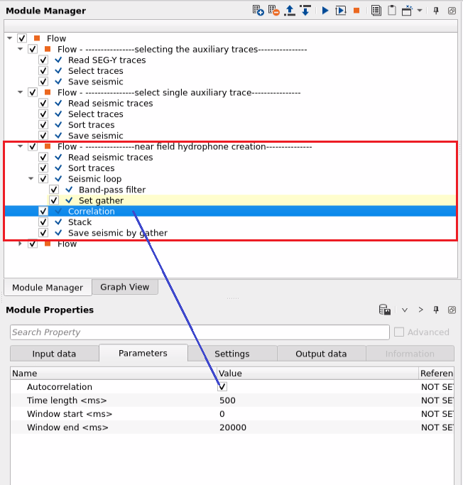
6.Next, do the auto-correlation of the output from the Set gather by using "Correlation" module.
7.Now stack all the auto-correlated outputs from the previous step to create a single wavelet by using "Stack" module. This is our Near Field Hydrophone (NFH) wavelet.
8.Finally, save the output from Stack module by using "Save seismic by gather" module.
Debubbling of the input data using Near Field Hydrophone
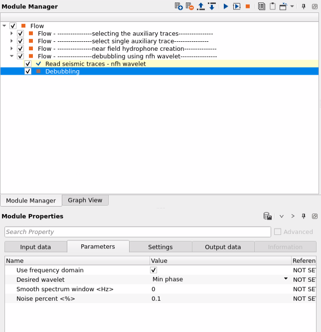
1.Read the Near Field Hydrophone (NFH) wavelet by using "Read seismic traces" module. Make sure to "Load data to RAM" as YES.
2.Connect/reference the Input DataItem of "Debubbling" module to Output gather of "Read seismic traces" module. Also, reference the Input wavelet to "Read seismic traces" output gather.
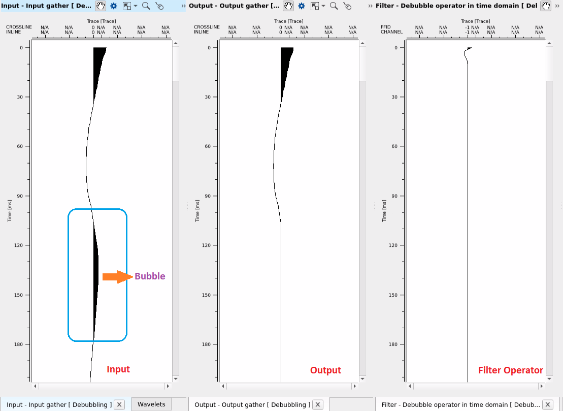
3.Execute the Debubbling module by double clicking on it or press the execute button to get the bubble free output along with Debubbling filter operator in time domain. Here is an example flow and the corresponding output(s).
![]()
![]()
Auto-connection - By default Yes (Checked)
Bad data values option { Fix, Notify, Continue } - This is applicable whenever there is a bad value or NaN (Not a Number) in the data. By default Notify. While testing, it is good to opt as Notify option. Once we understand the root cause of it, the user can either choose the option Fix or Continue. In this way, the job won't stop/fail during the production.
Number of threads - One less than total no of nodes/threads to execute a job in multi-thread mode.
Skip - By default, No (Unchecked). This option helps to bypass the module from the workflow.
![]()
![]()
Output gather - The debubbled seismic data gather with the bubble effect suppressed and the wavelet converted to the selected phase (minimum phase or zero phase). Connect this output to the next processing module in your workflow, such as a predictive deconvolution or band-pass filter.
Input wavelet gather - A diagnostic output showing the input source wavelet as received by the module, after any resampling to match the data sample rate but before filter application. Use the Wavelets vista view to compare this against the debubbled wavelet to verify the quality of bubble suppression.
Debubbled wavelet - The target wavelet after bubble removal — the result of applying the Wiener designature filter to the input wavelet. This is the desired phase shape (minimum phase or zero phase) that the output seismic traces will approximate. Inspect this wavelet in the Wavelets vista view to confirm that bubble oscillations have been eliminated and the wavelet is compact and well-shaped.
Debubble operator in time domain - The debubble filter operator represented in the time domain (obtained by inverse FFT of the frequency-domain filter). Inspect this in the Filter vista view to assess the temporal character of the operator. A well-designed operator should be compact and causal; a long, oscillatory operator may indicate that the Noise percent is too low or that the input wavelet needs smoothing or tapering.
![]()
![]()
YouTube video lesson, click here to open [VIDEO IN PROCESS...]
![]()
![]()
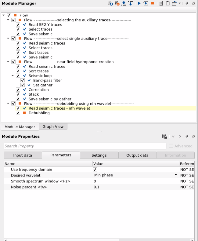
Here is an example workflow. In this flow, we've generated the near field hydrophone from the input field data. Each step of the workflow is explained in the "Creating wavelet from the input data" section. In case, far field signature is available then the user can use only the last step of "debubbling using nfh wavelet" workflow. In the place of NFH wavelet, the user uses the far field signature.
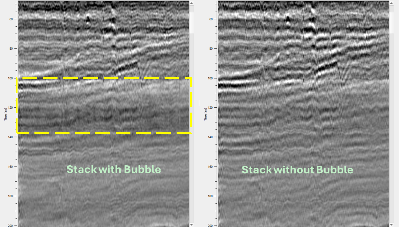
Here is an example stack section before and after Debubble.
![]()
![]()
Yilmaz. O., 1987, Seismic data processing: Society of Exploration Geophysicist
 * * * If you have any questions, please send an e-mail to: support@geomage.com * * *