![]()
![]()
QC attributes - post stack module is designed to display color maps of various calculated attributes, alongside a frequency spectrum of a post-stack data. The attributes are calculated inside the area defined by the analysis window and inside the noise analysis window. For QC attributes - post stack, the user can connect/reference the Horizons to do the analysis within the horizons for both signal and noise.
How To Use:
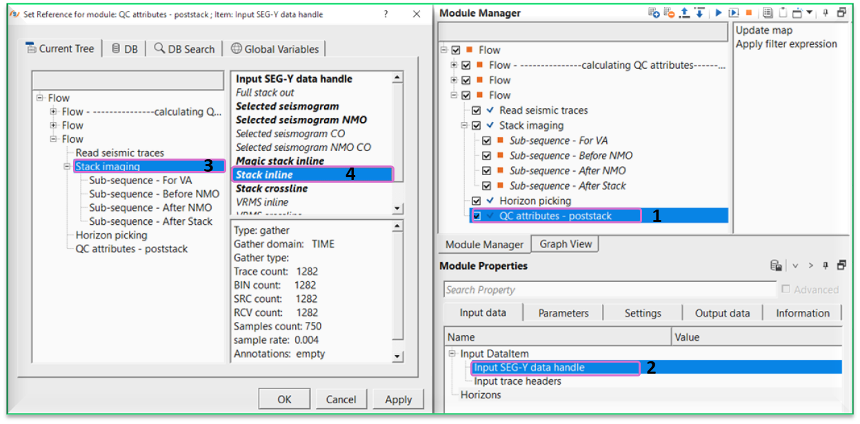
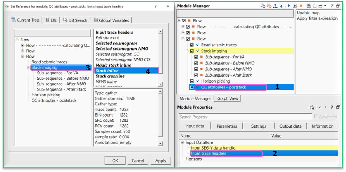
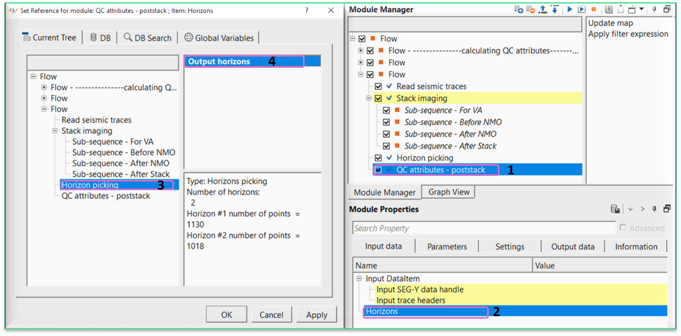
1)Connect the module to SEG-Y data handle and Output trace headers. Also, Output horizons to Horizons.
2)Output the vistas from the module (Location map, output , spectrum)
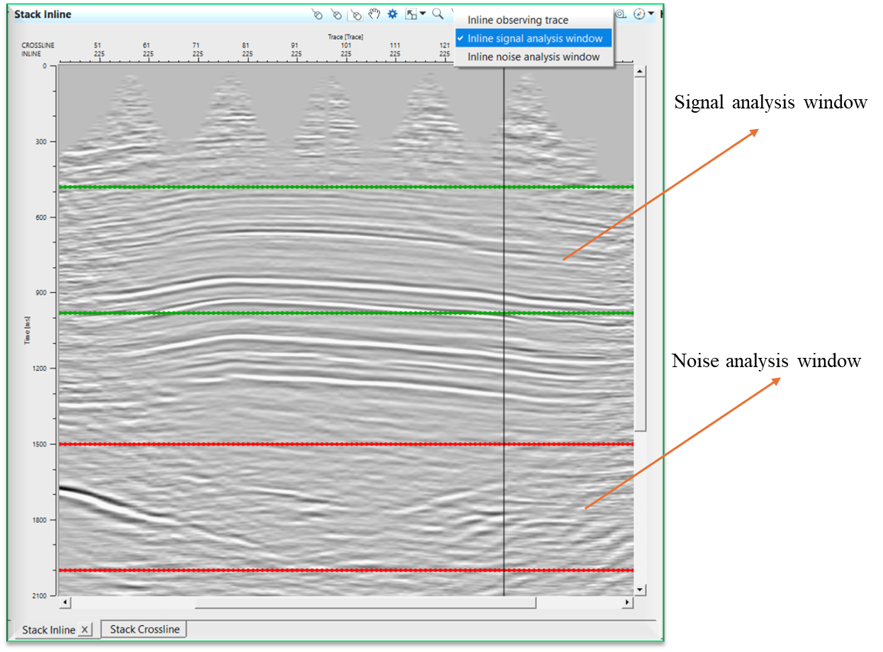
3)On the Output gather, adjust the Analysis window and the Noise analysis window to cover the portion of the data that you would like to analyze
4)You may do this by clicking on the ![]() icon, and turning on the interactive items for Analysis window and Noise Analysis window.
icon, and turning on the interactive items for Analysis window and Noise Analysis window.
Select any one of the windows from the control item icon. Here we are showing Analysis window (Signal window).
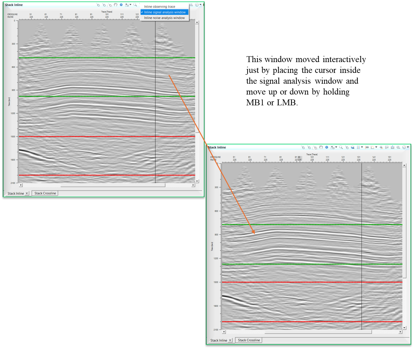
Now move/place the cursor inside the Signal analysis window (Green rectangle). A + icon appears. Now hold MB1 or LMB and move the window wherever the user wants to analyze the data. Now this window (Green rectangle) is the new Analysis window. Likewise, the user can perform Noise Analysis also.
5)Alternately, you may define these boxes by setting the extents for these two boxes under “Signal calculation window” and “Noise Calculation window” under the parameters tab
6)Choose the attributes you would like to calculate by ensuring they are checked off under “attributes”
7)Run the module to calculate attributes
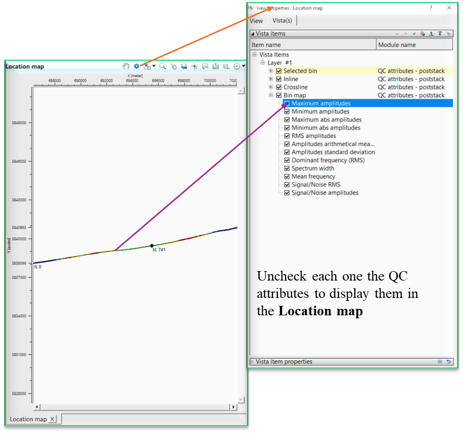
8)On the location map, open the View properties ![]() Choose which attribute you would like to see displayed as a color map by checking it off in the Attribute Map list:
Choose which attribute you would like to see displayed as a color map by checking it off in the Attribute Map list:
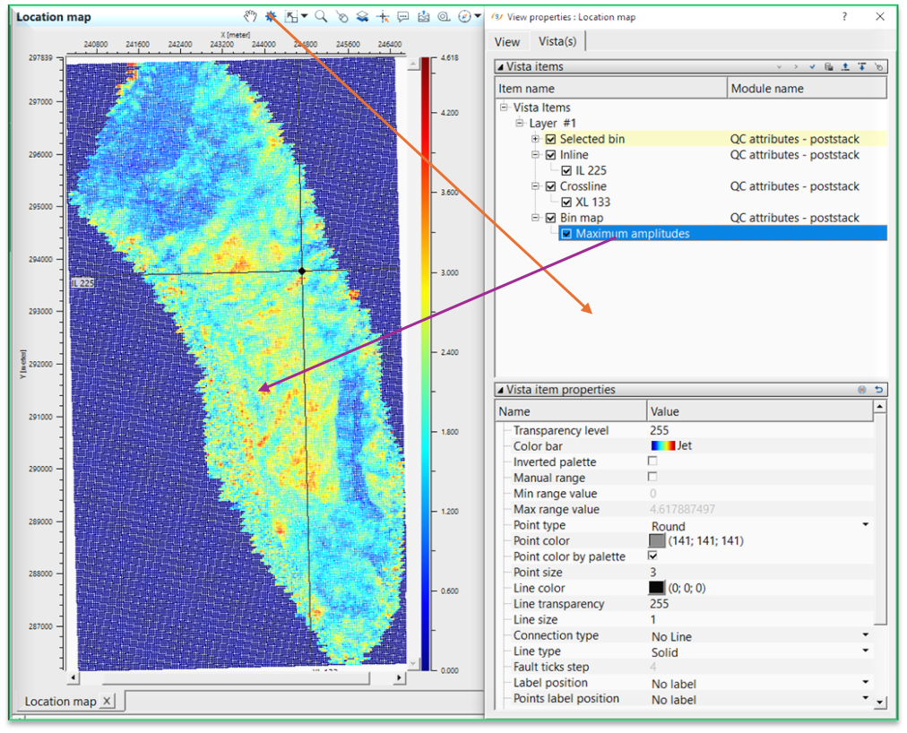
9)If the user wants to see a colour bar, make sure the user turn on “colour bar enabled “ in the view properties for the location map. The colour bar will be displayed for the currently highlighted vista item.
![]()
![]()
Input DataItem
Input SEG-Y data handle - this should be post-stack dataset only. Connect/reference to the Output SEG-Y data handle.
Input trace headers - connect/reference to the Output trace headers.
Horizons - Connect/reference to Output horizons. These horizons are used to define the signal and noise analysis windows on the basis of horizons which acts as starting and ending windows.
![]()
![]()
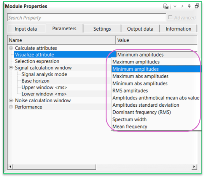
Calculate attributes - this section deals with attribute calculation. Select the desired/required attributes. By default, it will select and calculate all the available attributes from the list.
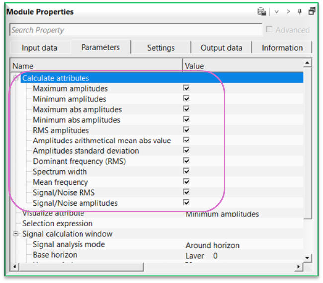
Maximum amplitudes - returns the highest positive amplitude value within the selected time window. Useful for detecting strong reflections or amplitude clipping.
Minimum amplitudes - returns the lowest (most negative) amplitude value within the selected window.
Maximum abs amplitudes - returns the largest amplitude magnitude regardless of polarity. Useful for identifying extreme signal or noise spikes.
Minimum abs amplitudes - returns the smallest amplitude magnitude within the selected window. Useful for detecting dead or muted traces.
RMS amplitudes - calculates the root-mean-square amplitude within the selected window. Represents overall signal energy.
Amplitudes arithmetical mean abs value - computes the average of absolute amplitudes. Provides a stable measure of average signal strength.
Amplitudes standard deviation - measures the variability of amplitudes around the mean. Higher values indicate greater amplitude fluctuations.
Dominant frequency (RMS) - calculates energy-weighted RMS frequency of the amplitude spectrum. Represents the dominant frequency content of the trace.
Spectrum width - measures spectral bandwidth around the mean frequency. Indicates frequency spread and resolution potential.
Mean frequency - calculates the amplitude-weighted average frequency of the trace spectrum.
Signal/Noise RMS - computes the ratio of RMS amplitude inside the signal window to RMS amplitude inside the noise window.
Signal/Noise amplitudes - calculates amplitude ratio between signal and noise windows. Higher values indicate cleaner data.
Visualize attribute { Maximum amplitudes, Minimum amplitudes, Maximum abs amplitudes, Minimum abs amplitudes, RMS amplitudes, Amplitudes arithmetical mean abs value, Amplitudes standard deviation, Dominant frequency (RMS), Spectrum width, Mean frequency, Signal/Noise RMS, Signal/Noise amplitudes } - displays the current calculated attribute as a map. By default, Maximum amplitude.
Bulk read size - specifies the total number of traces to read as a bulk.
Selection expression -
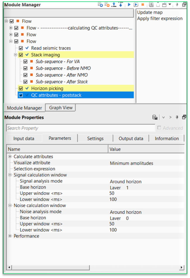
Signal calculation window - this section deals with signal calculation window.
Signal analysis mode { Internal, Around horizon } - select the analysis mode from the drop down menu. By default, Internal.
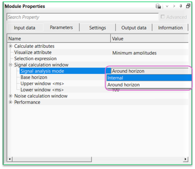
Signal analysis mode - Internal
Start type { Constant time, Horizon, Map } - there are 3 type of options available for start time. Select one of them from the drop down menu. By default, Constant time.
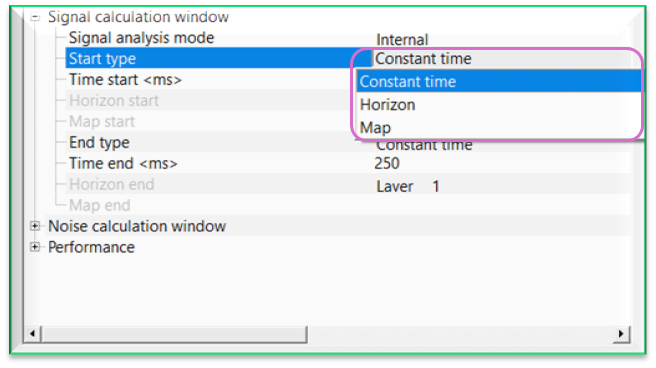
Time start - defines the beginning time (in ms) of the calculation window. Samples before this time are excluded from attribute computation.
Time end - defines the ending time of the calculation window. Samples after this time are excluded from calculations.
Horizon start { Layer___0, Layer___1 } - select the horizon from the drop down menu. The selected horizon acts as a start time window for signal analysis.
Horizon end { Layer___0, Layer___1 } - select the horizon from the drop down menu. The selected horizon acts as a end time window for signal analysis.
Map start - connect/reference to any map which can be used as a starting time. This map can be a topography map etc.
End type { Constant time, Horizon, Map }
Map end - connect/reference to any map which can be used as a ending time. This map can be a topography map etc.
Signal analysis mode - Around horizon - this option allows the user to analyze the signal within user defined base horizon with a lower and upper limits.
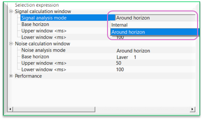
Base horizon { Layer___0, Layer___1 } - select the base horizon.
Upper window - this will acts as a upper window from the base horizon. By default, 50 ms which means the signal analysis window starts 50 ms above the base horizon.
Lower window - - this will acts as a lower window from the base horizon. By default, 50 ms which means the signal analysis window starts 50 ms below the base horizon.
Noise calculation window - this section deals with noise calculation window.
Noise analysis mode { Internal, Around horizon } - select the analysis mode from the drop down menu. By default, Internal.
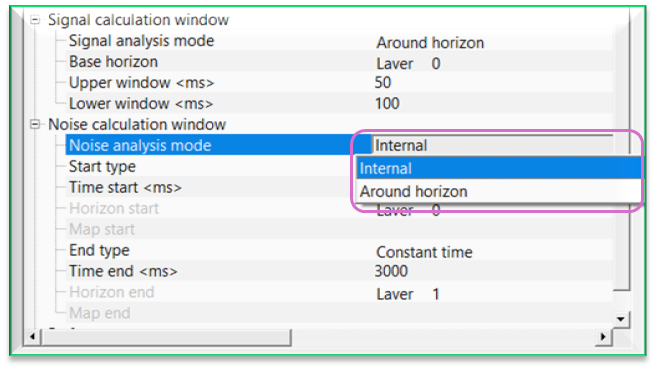
Noise analysis mode - Internal
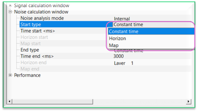
Start type { Constant time, Horizon, Map } - there are 3 type of options available for start time. Select one of them from the drop down menu. By default, Constant time.
Time start - defines the beginning time (in ms) of the calculation window. Samples before this time are excluded from attribute computation.
Time end - defines the ending time of the calculation window. Samples after this time are excluded from calculations.
Horizon start { Layer___0, Layer___1 } - select the horizon from the drop down menu. The selected horizon acts as a start time window for noise analysis.
Horizon end { Layer___0, Layer___1 } - select the horizon from the drop down menu. The selected horizon acts as a end time window for noise analysis.
Map start - connect/reference to any map which can be used as a starting time. This map can be a topography map etc.
End type { Constant time, Horizon, Map }
Map end - connect/reference to any map which can be used as a ending time. This map can be a topography map etc.
Noise analysis mode - Around horizon - this option allows the user to analyze the noise within user defined base horizon with a lower and upper limits.
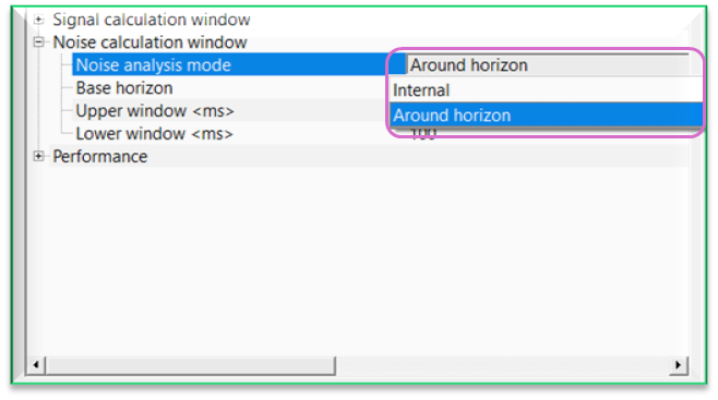
Base horizon { Layer___0, Layer___1 } - select the base horizon.
Upper window - this will acts as a upper window from the base horizon. By default, 50 ms which means the noise analysis window starts 50 ms above the base horizon.
Lower window - this will acts as a lower window from the base horizon. By default 50 ms which means the noise analysis window ends 50 ms below the base horizon.
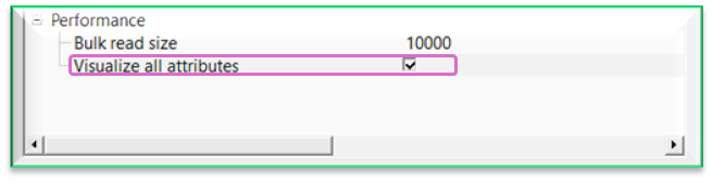
Performance - this section deals with total number of traces to read at a time as a bulk and displaying the calculated QC attributes all of them at once or not.
Bulk read size - specify the total number of traces to read as a bulk at one time. By default, 1000.
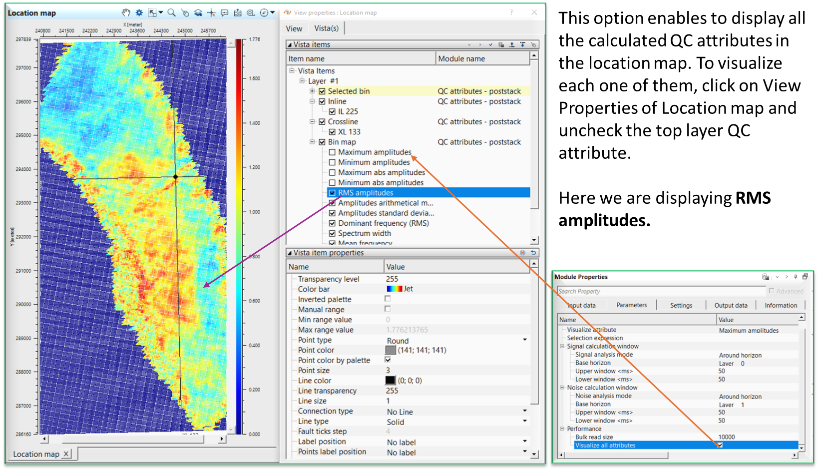
Visualize all attributes - displays all the calculated QC attributes in the Location map. By default, FALSE (Unchecked). If it is TRUE (Checked), it will display all the calculated QC attributes one below the other in the location map under Bin map.
![]()
![]()
Auto-connection - By default, TRUE(Checked).It will automatically connects to the next module. To avoid auto-connect, the user should uncheck this option.
SEG-Y read params - parameters for setting advanced parameters of reading seismic traces from disk.
Thread count (for SSD) - amount of treads for reading seismic traces from disk.
Bulk size (traces) - size of a chunk (data portion) for reading seismic traces from disk.
Number of threads - One less than total no of nodes/threads to execute a job in multi-thread mode. Limit number of threads on main machine.
Skip - By default, FALSE(Unchecked). This option helps to bypass the module from the workflow.
![]()
![]()
Output calculated attributes - outputs the QC attributes as an output
Traces selected by attribute - generates the traces selected by the attributes.
Number of selected traces - displays the total number of trace selected as an information.
![]()
![]()
In this example workflow, we are showing how to perform QC attribute analysis for a post stack dataset. For this workflow, we need the post stack dataset (2D or 3D). Along with it, Horizons. These horizons are not mandatory however, if the user wants to perform the QC attribute analysis within horizons then it is required.
For this workflow, make the necessary connections.
It is not mandatory to follow the above mentioned workflow for QC attributes - poststack module calculation. In this we've used Read seismic traces and Stack Imaging followed by Horizon picking. The objective of the 1st two modules is to create a stack section. In the 3rd module i.e. Horizon picking, we take Stack inline from Stack Imaging module to the Horizon picking module as an input and pick the horizons of this stack inline.
If the user have the stack and horizons then they can use other alternative workflow like read seismic traces to read the stack/stack volume and Import post stack horizons module to connect/reference to the QC attributes - poststack module.
After necessary connections/reference, adjust the parameters and choose the appropriate QC attributes & calculation windows in the Parameters tab.
Execute the module and generate the Vista items.
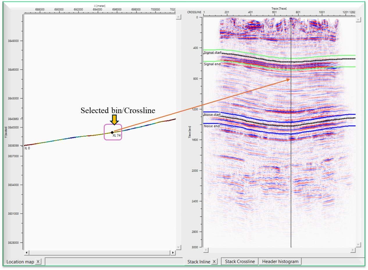
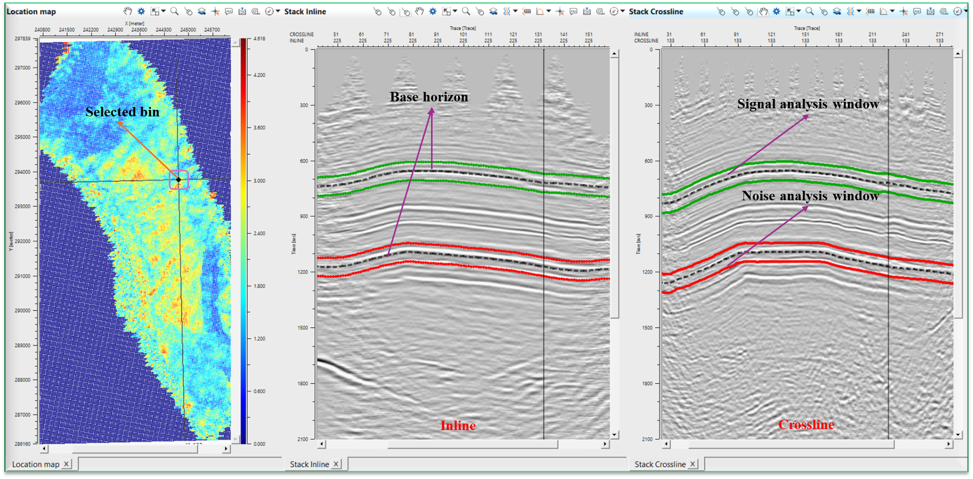
In the above image, we can observe Signal analysis window & Noise analysis window. In between Signal analysis window, we observe a black dotted line which is nothing but the horizon. Just above and below this horizon, there are two lines which are used to a reference to calculate the attributes + or 1 user defined value from the horizon.
Likewise, Noise analysis window is represented with a horizon and two lines above and below the horizon.
In the Performance section of the Parameters tab, Visualize all attributes option is FALSE (Unchecked). If the user wants to see all the attributes on the Location map, make it TRUE (Checked).
In case of 3D dataset, we follow the same process.
![]()
![]()
Update map - this will refresh the location map in case it is not properly displayed or update the display when the user changed the different attributes.
Apply filter expression - this is applicable when the user used "selection expression" parameter to filter any of the attributes. This will perform that task.
![]()
![]()
YouTube video lesson, click here to open [VIDEO IN PROCESS...]
![]()
![]()
Yilmaz. O., 1987, Seismic data processing: Society of Exploration Geophysicist
 * * * If you have any questions, please send an e-mail to: support@geomage.com * * *
![]()