Pre Stack Depth Migration via Kirchhoff algorithm (PSDM stage)
![]()
![]()
Note: This module is deprecated. For new projects, use the current Kirchhoff PreSDM modules. Existing workflows that reference this module will continue to function, but no further development will be applied to it.
Kirchhoff depth migration is a fundamental algorithm in seismic data processing used to reconstruct subsurface images by mapping recorded seismic data to their true spatial locations in depth. The method is based on the Kirchhoff integral solution to the wave equation and assumes that seismic waves can be treated as high-frequency approximations propagating through the subsurface. It requires an accurate velocity model and the calculation of travel times for each source-receiver pair.
The algorithm uses the Kirchhoff integral equation to represent the seismic wavefield:
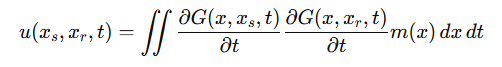
where:
• u(Xs, Xr, t) is the recorded seismic data,
• G(X, Xs, t) and G(X, Xr, t) are Green's functions describing the travel time from the source (Xs) and receiver (Xr) to the subsurface point (X),
• m(X) is the reflectivity model being reconstructed.
Kirchhoff migration involves summing the contributions of seismic energy along isochron surfaces, defined by the travel time equation:
![]()
where T(X, Xs) and T(X, Xr) are the travel times from the subsurface point to the source and receiver, respectively. The reflectivity at a given point is determined by stacking the seismic amplitudes along these surfaces. This process is computationally intensive, requiring accurate travel-time tables and an efficient summation scheme.
Kirchhoff depth migration is particularly effective in areas with relatively simple subsurface structures or where a good initial velocity model is available. The algorithm's flexibility allows it to handle varying offsets and irregular acquisition geometries. However, its accuracy depends on the resolution of the velocity model and the correct computation of travel times, making iterative velocity model updates a crucial part of the workflow.
![]() The module requires travel time file as input data, therefore please be sure that it was calculated before via Time table calculation for tomo update module.
The module requires travel time file as input data, therefore please be sure that it was calculated before via Time table calculation for tomo update module.
![]()
![]()
Use trace vector on disk - enable this option when the trace header dataset is too large to hold in RAM. When enabled, all trace headers are read directly from disk on demand, reducing memory usage at the cost of additional I/O. In this mode, connect the Input traces data handle item instead of the in-memory Input data trace headers.
Input SEG-Y data handle - connect to the input SEG-Y data handle. The input seismic must be pre-migration regularized gathers or COMF (Common Offset Migration Friendly) enhanced gathers, without NMO corrections applied. The data should be in the time domain prior to migration.
Input data trace headers - connect to the input trace header item. This carries the geometry information (shot/receiver positions, CDP, offset) associated with the pre-migration gathers. Used when trace headers are loaded into memory (i.e., when Use trace vector on disk is disabled).
Input trace data handle - active only when Use trace vector on disk is enabled. In that mode, trace headers are read directly from disk instead of being held in RAM, which is necessary when the trace header dataset is too large to fit in memory.
Depth velocity (to find optimal params) - optional input. When connected, the depth velocity model is used to extract datum elevation information from trace headers, which helps the migration correctly account for surface topography. If the Datum parameter is set manually, this input can be left unconnected.
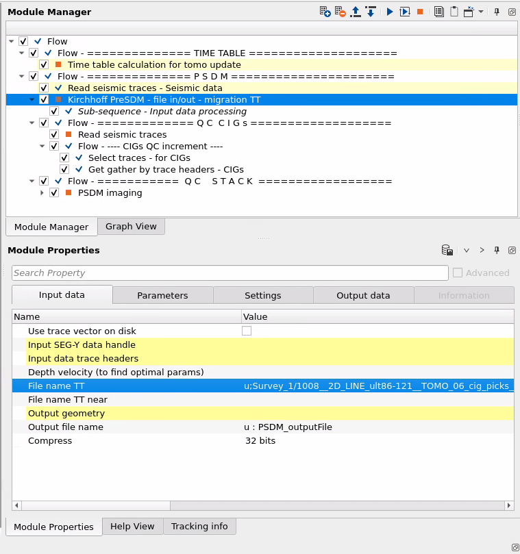
File name TT - path to the precomputed travel time table file (extension .ttfile). This file must be calculated in advance using the Time table calculation for tomo update module. The travel time tables store the two-way travel times from every source/receiver surface position to every subsurface image point in the depth model.
File name TT near - path to the precomputed travel time table file computed specifically for near-offset imaging. Used only when Use near offset TT is enabled. Near-offset travel time tables can be computed with a separate run of the Time table calculation for tomo update module configured for near offsets.
Output geometry - defines the spatial grid for the output migrated Common Image Gathers (CIGs). Connect a bin grid item derived from an input stack, gather dataset, or velocity model to define the output bin locations. All migrated traces will be organized into this output geometry.
Output file name - file path and name for the output Common Image Gathers (CIGs) written in GSD format. The CIGs contain the depth-migrated seismic data organized by offset or offset-vector tile, and are used for subsequent velocity model quality control and tomographic updating.
Compress - bit depth for the output CIG file storage. Options are 32 bits (full floating-point precision, largest file size), 16 bits (half precision, smaller files with minor amplitude precision loss), or 8 bits (minimum file size, suitable only for QC purposes where amplitude fidelity is not critical). For production workflows use 32 bits.
![]()
![]()
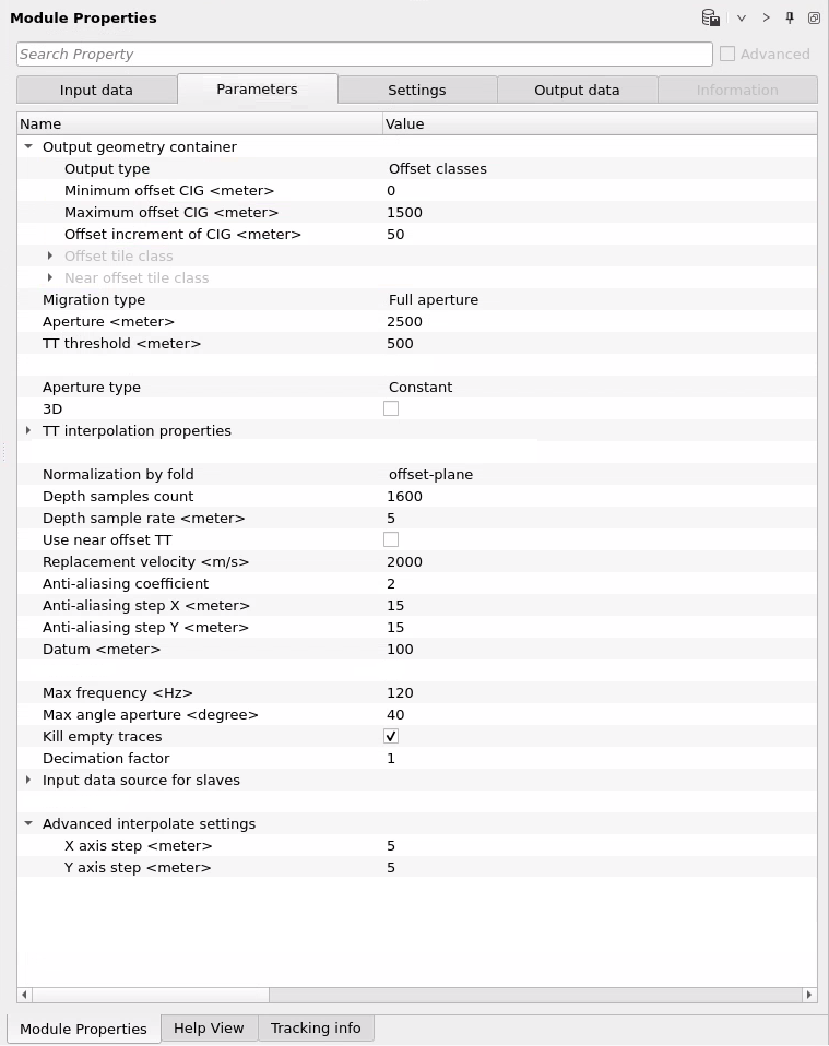
Output geometry container : defines the offset structure of the output Common Image Gathers. This group controls how many offset traces each CIG contains and the spacing between them. The configuration here determines whether output CIGs are organized by absolute offset (Offset classes), by variable offset ranges, or by offset-vector tile (OVT) for azimuthal analysis.
Output type - output type of offsets: Offset classes (simple offset definition), Offset tile classes (for COV/OVT - Common Offset Vector/Offset Vector Tile), Offset tile classes 2 (for COV/OVT - Common Offset Vector/Offset Vector Tile with an extra option for near offset definition).
Offset class:
Minimum offset CIG - the smallest source-receiver offset (in meters) that will be included in the output CIGs. Set to 0 m (default) to include near-offset traces from zero offset. Increasing this value excludes shallow-angle contributions and may suppress guided wave noise.
Maximum offset CIG - the largest source-receiver offset (in meters) included in the output CIGs. Default is 3000 m. Set this to match the maximum usable offset in the acquisition, typically limited by the maximum offset available in the input gathers.
Offset increment of CIG - the interval in meters between successive offset traces in each CIG. Default is 100 m. A smaller step produces more densely sampled CIGs for detailed velocity analysis, at the cost of increased output data volume.
Offset tile class:
Inline offset from - provide the minimum offset in meters for generating the OVT output in inline direction.
Inline offset to - maximum offset in meters for generating the OVT output in inline direction.
Inline offset step - step offset in meters for generating the OVT output in inline direction.
Xline offset from - provide the minimum offset in meters for generating the OVT output in xline direction.
Xline offset to - maximum offset in meters for generating the OVT output in xline direction.
Xline offset step - step offset in meters for generating the OVT output in xline direction.
Near offset tile class:
Near inline offset from - provide the minimum offset in meters for generating the OVT output in inline direction for NEAR offsets only.
Near inline offset to - maximum offset in meters for generating the OVT output in inline direction for NEAR offsets only.
Near inline offset step - step offset in meters for generating the OVT output in inline direction for NEAR offsets only.
Near xline offset from - provide the minimum offset in meters for generating the OVT output in xline direction for NEAR offsets only.
Near xline offset to - maximum offset in meters for generating the OVT output in xline direction for NEAR offsets only.
Near xline offset step - step offset in meters for generating the OVT output in xline direction for NEAR offsets only.
Migration type :
Full aperture - the entire migration aperture. Conventional migration option (use it by default).
CMP partial summed - migration aperture CMP partial summed (advanced option).
CMP partial non-summed - migration aperture CMP partial non-summed (advanced option).
Aperture - the half-aperture radius (in meters) of the Kirchhoff migration operator. Default is 3000 m. This means that for each output image point, seismic contributions from input traces within a circle of this radius are summed. A larger aperture captures more energy from steeply dipping reflectors but increases computation time and can introduce migration noise if set too large. Note: this value is the half-distance (radius), not the full diameter.
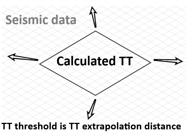
TT threshold - the margin distance (in meters) beyond the boundary of the computed travel time table area within which extrapolation is permitted. Default is 1000 m. When the seismic data coverage extends slightly beyond the area covered by the TT tables, the module can extrapolate travel times into this margin rather than skipping those traces. Setting this value too large may introduce extrapolation artefacts near model boundaries. See the diagram below:
Aperture type - controls how the migration aperture varies with depth. Choose Constant to apply the same aperture radius at all depths, or Depth variant to define a table of depth-aperture pairs where the aperture increases with depth. In most cases a Depth variant aperture is preferable: shallow targets require smaller apertures (to reduce noise) and deeper targets benefit from larger apertures (to capture wide-angle reflections). When Depth variant is selected, populate the Depth-aperture factors table with at least two entries.
3D - enable this flag when processing 3D seismic data. When enabled, the migration operator searches for contributions in both the inline and crossline directions within the aperture radius. For 2D lines, leave this unchecked so that the migration operator is constrained to the 2D profile plane.
TT interpolation properties - controls how travel times are interpolated from the discrete TT table grid onto the actual source/receiver positions of the input traces. When input trace positions do not coincide exactly with TT table grid nodes, interpolation is needed to estimate the travel time at that position. Four methods are available (see Interpolation method below). Triangulation is the default and is recommended for most cases; Kriging provides statistically optimal results when data is unevenly sampled; Bilinear is fast but only valid on regular grids; Nearest is the simplest approach and introduces staircase artefacts at low TT table resolutions.
Interpolation method :
Triangulation - triangulation interpolation is a mathematical method used to estimate values at unknown points. The method divides the spatial domain (e.g., depth slices or grid cells in the velocity model) into a network of non-overlapping triangles (in 2D) or tetrahedra (in 3D), where the vertices represent points with known travel times. Within each triangle or tetrahedron, the travel time at an unknown point is interpolated linearly using the known travel times at the vertices. The interpolation assumes that the travel time changes linearly across the triangle or tetrahedron.
Kriging - unlike triangulation, kriging assumes a spatial correlation structure between the points and uses this relationship to provide a statistically optimal estimate, incorporating both the spatial distribution of data points and their values.
Bilinear - bilinear interpolation is a simple and fast method used to estimate travel times at unknown points within a regular 2D grid based on the travel times at four surrounding grid points. It assumes that the travel time varies linearly along both the X and Y directions.
Nearest - nearest-neighbor interpolation is the simplest method for estimating travel times at unknown points. It assigns the travel time of the closest known data point to the unknown point without considering gradual changes or trends between data points.
Kriging covariance type - the covariance type refers to the mathematical model used to describe the spatial correlation between data points. This covariance model plays a crucial role in defining how the values at different locations are statistically related, which directly impacts the interpolation results.
Exponential - Suitable for data with rapidly decreasing spatial correlation. Correlation diminishes exponentially with distance but never truly reaches zero.
Spherical - A commonly used covariance type that assumes the spatial correlation increases up to a certain distance (called the range), beyond which points are uncorrelated. The correlation gradually decreases as the distance approaches the range.
Gaussian - Represents a smooth, gradual decrease in correlation, often used for very continuous data.
Kriging range -parameter of the variogram or covariance model that defines the maximum distance over which spatial correlation exists between data points. Beyond the range, the values at different locations are considered uncorrelated or independent.
Kriging number of points - refers to the number of nearby data points used to estimate the value at an unknown location during the interpolation process. This parameter controls how many known values in the vicinity of the target point are included in the kriging calculation.
Normalization by fold - controls how output amplitudes are normalized to account for uneven fold distribution across the migrated volume. Options are: none (no normalization applied); trace (divides each output trace amplitude by the number of input wavefronts that contributed to that trace, correcting for trace-level fold variation); sample (divides each individual depth sample by the number of wavefronts that contributed at that sample, providing the finest-grained normalization); offset-plane (default, normalizes by the fold within each offset class plane, balancing amplitudes between near and far offset CIG traces). Use offset-plane for most production workflows; use sample for detailed amplitude analysis in areas of variable fold.
Depth samples count - the total number of depth levels in the output migrated volume. Default is 1000. The maximum imaging depth equals Depth samples count multiplied by Depth sample rate. For example, 1000 samples at 5 m/sample gives a maximum imaging depth of 5000 m. Increase this value to image deeper targets.
Depth sample rate - the vertical spacing between depth samples in the output migrated image, in meters. Default is 5 m. This defines the vertical resolution of the output CIGs. A smaller interval improves vertical resolution but increases output data volume and computation time. The value should be consistent with the wavelength of the dominant seismic frequency — typically one-quarter to one-eighth of the minimum wavelength.
Use near offset TT - when enabled, the migration uses a separate set of travel time tables computed specifically for near-offset traces. This is useful when the near-offset acquisition geometry differs from the full-offset geometry and standard TT tables do not adequately represent the near-offset wavefield. When this option is enabled, connect the File name TT near input with travel time tables computed for the near-offset geometry.
Replacement velocity - the constant velocity (in m/s) used to propagate seismic energy between the acquisition datum and the surface topography. Default is 1500 m/s (minimum 150 m/s). This value should match the near-surface velocity used when the travel time tables were computed. An incorrect replacement velocity introduces static shifts in the migrated depth image.
Anti-aliasing coefficient - is a parameter used to prevent aliasing artifacts during the migration process, particularly when data is sampled at a resolution that is insufficient to accurately represent high-frequency wavefields. Aliasing occurs when higher-frequency components are incorrectly reconstructed as lower frequencies due to undersampling, which can distort the final seismic image. The anti-aliasing coefficient helps mitigate this issue by applying frequency-dependent filtering during the migration process. Choose between 0 and 1. Zero means no anti-aliasing.
Anti-aliasing step X - antialiasing bin step in X direction, increase bin size to increase antialiasing effect.
Anti-aliasing step Y - antialiasing bin step in Y direction, increase bin size to increase antialiasing effect.
Datum - the reference elevation (in meters) from which depth migration is applied. Default is 1100 m. Unlike PreSTM (which migrates from topography), PreSDM migration requires a flat datum from which the travel times were computed. Set this to the datum elevation used during travel time table computation. An inconsistency between this value and the TT file datum will cause depth errors in the migrated output.
Max frequency - the upper frequency limit (in Hz) used during the migration process. Default is 120 Hz. Frequencies above this value are excluded during the Kirchhoff summation, which acts as a low-pass filter and reduces migration noise. Set this to match the highest usable frequency in your seismic bandwidth. Lowering this value improves noise suppression but reduces vertical resolution.
Max angle aperture - the maximum dip angle (in degrees) of reflectors to include in the migration summation. Default is 80 degrees. Restricting this angle excludes steeply dipping events that are poorly constrained by the acquisition geometry, reducing migration noise from operator aliasing. For structurally complex areas with steep dips, set this value higher. For simpler geology, a value of 60-70 degrees is often sufficient.
Kill empty traces -when enabled (default), output CIG traces that contain no migrated energy (all zeros) are automatically removed from the output file. This reduces output file size and avoids confusion in downstream QC. Disable this option if you need to preserve the full output grid geometry including empty locations.
Decimation factor - reduces the number of input traces processed by keeping only every N-th trace (default is 1, meaning all traces are used). Setting a Decimation factor greater than 1 speeds up test runs when evaluating migration parameters. For example, a value of 10 processes approximately one-tenth of the input data, enabling rapid parameter tests before committing to a full production run. Always reset to 1 for production migration.
Advanced params
Use local storage - when running in a cluster (distributed) environment, enable this option to write intermediate and output data to the local disk of each compute node rather than to shared network storage. This significantly improves I/O throughput and reduces network load during large-scale migrations.
Seismic filename - the full path and file name on the local disk of the compute node where intermediate migration output will be stored. Used only when Use local storage is enabled.
Advanced interpolate settings
X axis step - the grid step size (in meters) in the X direction used for the internal TT table interpolation grid. Default is 5 m. This controls the spatial resolution of the interpolated travel time field. A smaller step gives more accurate travel time estimates at the cost of additional memory and computation time. This setting does not change the output bin size, only the accuracy of the TT interpolation between the input table nodes.
Y axis step - the grid step size (in meters) in the Y direction used for the internal TT table interpolation grid. Default is 5 m. Functions the same as X axis step but in the crossline direction. For anisotropic bin geometries (inline spacing different from crossline), set X axis step and Y axis step independently to match the respective bin dimensions.
![]()
![]()
SegyReadParams - parameters for setting advanced parameters of reading seismic traces from disk:
Thread count (for SSD) - number of parallel threads used to read seismic traces from disk. Increasing this value can improve I/O throughput when reading from solid-state (SSD) storage. For spinning-disk (HDD) storage, setting too many threads may degrade performance due to seek overhead.
Bulk size (traces) - the number of traces read from disk in a single I/O operation. Larger bulk sizes reduce the number of disk access operations and generally improve throughput, at the cost of higher memory usage during reading. Tune this value based on available RAM and the typical gather size of the input data.
Execute on { CPU, GPU } - select which type of processor will be used for calculations: CPU or GPU.
Distributed execution - if enabled: calculation is on coalition server (distribution mode/parallel calculations).
Bulk size - chunk size is RAM in megabytes that is required for each machine on the server (find this information in the Information, also need to click on action menu button for getting this statistics):
Limit number of threads on nodes - limit numbers of of threads on nodes for performing calculations.
Job suffix - add an job suffix.
Set custom affinity - an axillary option to set user defined affinity if necessary.
Affinity - add your affinity to recognize you workflow in the server QC interface.
Number of threads - limit number of threads on main machine.
Run scripts - it is possible to use user's scripts for execution any additional commands before and after workflow execution:
Script before run - path to ssh file and its name that will be executed before workflow calculation. For example, it can be a script that switch on adn switch off remote server nodes (on Cloud).
Script after run- path to ssh file and its name that will be executed before workflow calculation.
Skip - disables this module so it is bypassed during workflow execution. Use this to temporarily exclude the migration step from a workflow without removing the module and its parameter settings.
![]()
![]()
Output geometry - the output geometry item generated after migration, available for downstream QC steps. Connect this to a geometry viewer or QC module to inspect the spatial coverage and fold of the migrated CIG dataset.
Dynamic time table - the dynamic (runtime-generated) travel time table item produced during migration. Connect this to a visualization module to display the travel time fields for QC purposes, verifying that the TT tables are correctly applied to the input geometry.

This module has no custom action buttons. Migration is triggered by the standard workflow Run command.
![]()
![]()
This module produces no VisualVista display items directly. Use the Output geometry and Dynamic time table output items to monitor results in downstream QC modules.
![]()
![]()
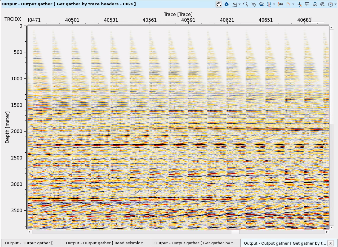
The entire workflow example with all necessary modules (travel time calculation, migration and QC).
As input data we need travel time tables, seismic gathers (no NMO-ed), output geometry we can get from the input seismic gathers:
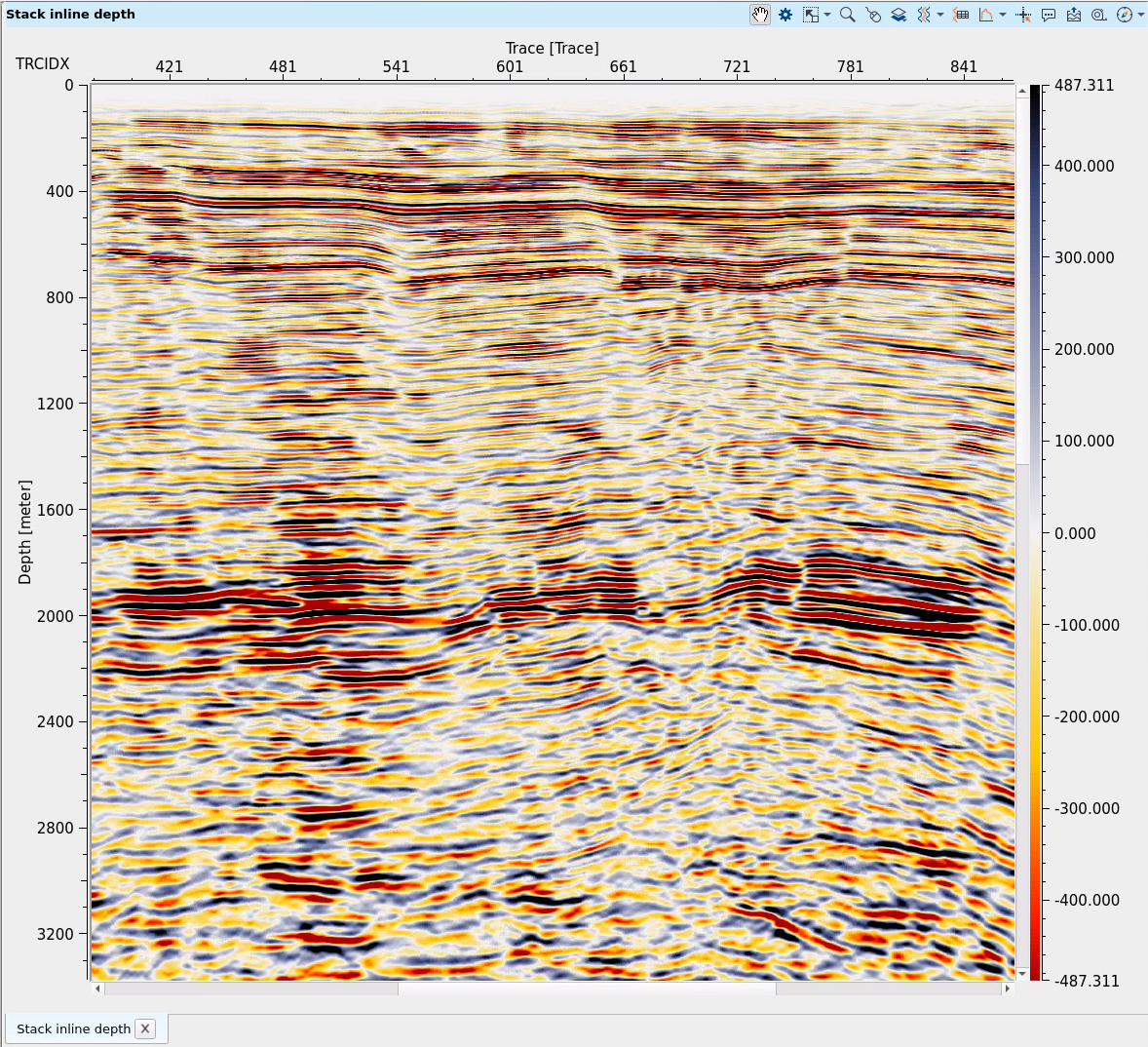
On the output we have migrated CIGs dataset, for QC we need to read it via Read seismic traces. For Stack please use PSDM imaging, it can create stack in depth and in time domains:
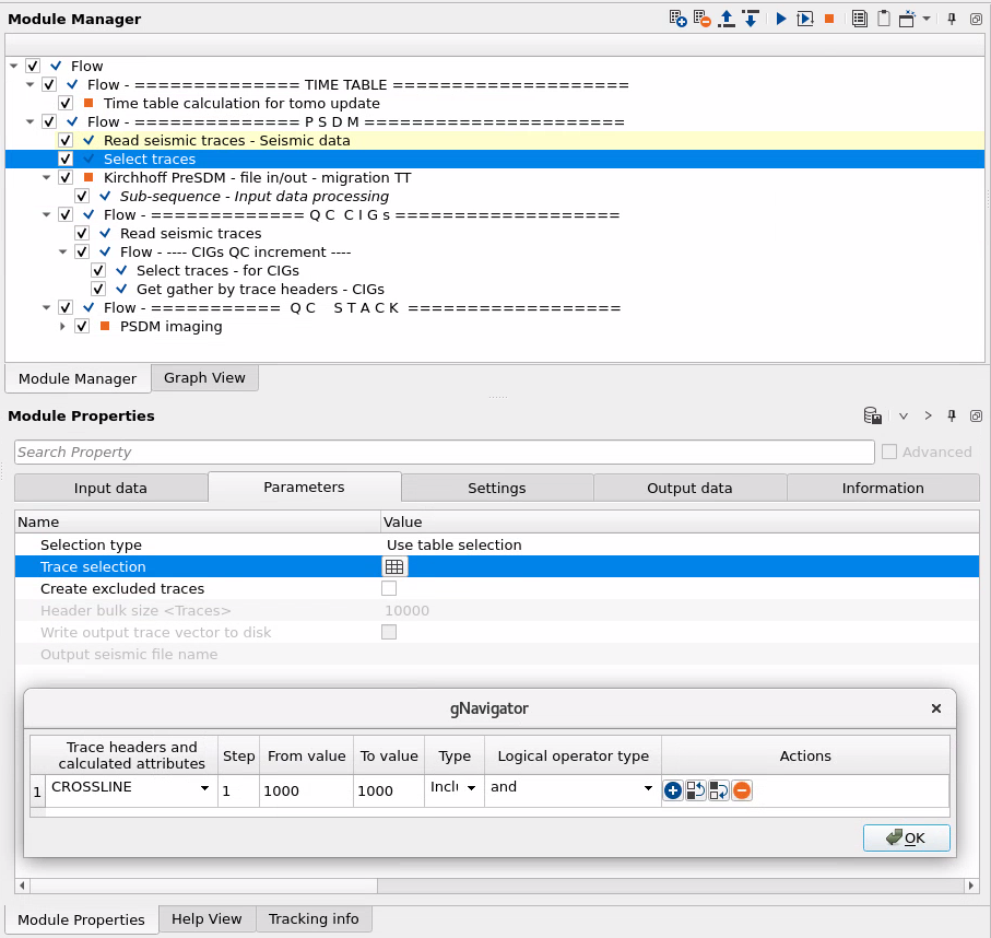
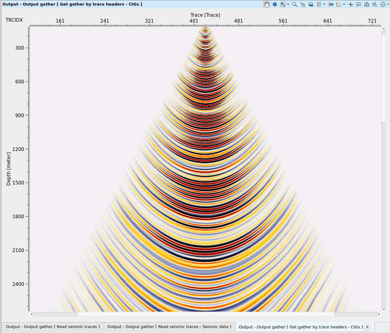
For the impulse response test we need to select one CMP from the input gathers and set ALL DATA WITHOUT SELECTION to the Output geometry:
![]()
![]()
 If you have any questions, please send an e-mail to: support@geomage.com