![]()
![]()
Onshore seismic data acquisition comes with many challenges. In many a times, the data is acquired in hilly terrains, agricultural lands, highly noisy city environments etc. Sometimes, the quality of the recorded data with respect to noise and amplitude is related to the poor coupling of the geophone. The amplitude quality compromises with the poor quality of geophones or the geophone may not functioning properly due to various reasons like the temperature which alter the mechanical properties of the geophone. This leads to distortion/alter of the amplitudes and frequency. Another reason for the poor quality of the amplitudes is the age of the geophone. Over a period of time, the geophone 's sensitivity goes down due to prolonged use of it in the field and regular wear and tear.
This module is designed to compensate for the amplitude response of geophones. It allows you to adjust the amplitudes based on the frequency. Proper compensation of the geophone results in stable geophone response and reliable data without any shifts or frequency distortions.
If the geophone' s frequency response starts to degrade (lower sensitivity for higher frequencies), the algorithm will adjust/compensate the frequency response to have an accurate frequency values at higher frequencies. Similarly, in case of the amplitude correction of the seismic data, the algorithm adjust/compensate the geophone's gain to get the amplitudes correctly/evenly.
The compensation is performed in the frequency domain. For each gather, the module transforms each trace to the frequency domain using a Fast Fourier Transform (FFT), applies a frequency-dependent gain correction defined by the user-supplied frequency-amplitude table (interpolated as a smooth spline curve), and then transforms the corrected trace back to the time domain. Only samples that are non-zero in the original trace are written back to the output, preserving dead trace masks.
The module belongs to the Deconvolution group and is typically applied during the pre-processing stage, before noise attenuation or deconvolution steps, so that subsequent processes work on amplitude-balanced data.
![]()
![]()
Input gather - provide the input gather. If it is within the seismic loop, it will automatically connects the previous modules output as an input for this module.
Connect the seismic gather to be corrected. This is typically a shot gather or CMP gather in time domain. When placed inside a seismic processing flow (sequence loop), the input connection is made automatically from the previous module's output.
![]()
![]()
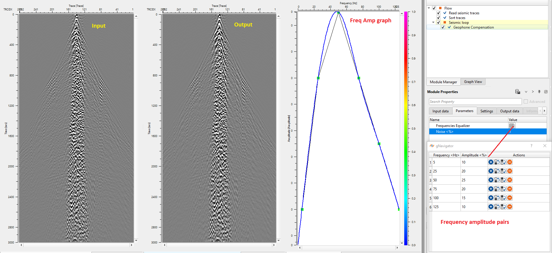
Frequencies Equalizer - Provide the frequency, amplitude pairs to compensate the amplitude with related to frequencies. Depending on the data quality, the user should provide the % amplitude compensation at various frequency ranges.
This table defines the frequency-dependent compensation curve. Each row specifies a control point with two values: Frequency (in Hz) and Amplitude (as a ratio). The module fits a smooth cubic spline through all the control points and applies the resulting curve as a frequency-domain gain correction to every trace.
An Amplitude value of 1.0 at a given frequency means no correction is applied at that frequency. Values greater than 1.0 boost that frequency band; values less than 1.0 attenuate it. For example, setting Amplitude to 2.0 at 10 Hz would double the spectral energy at 10 Hz, compensating for a geophone that records that frequency at half its true strength.
By default, four control points are provided at 10, 20, 45, and 75 Hz, all with Amplitude = 1.0 (no correction). You must supply at least two control points for the spline to be computed. Add more rows to shape the correction curve more precisely across the frequency band of interest. The frequency range should span from below the lowest signal frequency to above the highest usable signal frequency.
The compensation curve can also be edited interactively in the built-in Equalizer visualization panel, which displays the frequency-amplitude plot. Left-click to add or drag control points on the curve; right-click a control point to remove it. Changes made in the panel are immediately reflected in the table and vice versa. The Total spectrum panel shows the resulting gain curve interpolated at every output frequency bin, so you can preview the effect before running the job.
Noise - define the percentage white noise added to the data. This noise % stabilizes the output. By default 1%.
This parameter controls the stabilization floor for the frequency-domain inversion. Internally, the module applies a gain of 1 / max(compensation_value, noise_floor) at each frequency bin. Without this floor, any frequency where the user-defined compensation curve approaches zero would produce an extremely large — and numerically unstable — gain boost. The noise value prevents this by ensuring the denominator never falls below the specified fraction.
The default value of 1% is appropriate for most datasets. Increase this value (e.g., to 5–10%) if the output shows ringing or high-frequency amplification artifacts, which indicates that the compensation curve reaches very low values in some frequency band and requires stronger regularization. Decrease it only if you are confident the compensation curve is well-behaved (stays well above zero) across the entire frequency range.
![]()
![]()
Auto-connection - By default Yes (Checked)
When enabled, the module automatically connects its input and output gathers to the adjacent modules in the processing sequence. Leave this checked in normal use. Disable it only when you need to manually route data connections, for example when branching the flow or connecting a non-sequential data source.
Bad data values option { Fix, Notify, Continue } - This is applicable whenever there is a bad value or NaN (Not a Number) in the data. By default Notify. While testing, it is good to opt as Notify option. Once we understand the root cause of it, the user can either choose the option Fix or Continue. In this way, the job won't stop/fail during the production
Controls how the module responds when it encounters invalid sample values (NaN or infinity) in the input data. Three options are available:
Notify (default) — the job stops and reports the location of the bad value. Use this during testing to diagnose where bad data originates.
Fix — replaces bad values with zero before processing continues. Use this in production once you understand the cause and are confident replacement with zero is acceptable.
Continue — passes the bad values through without modification and keeps the job running. Use this when bad values are expected in a small number of traces and you do not want the job to stop.
Number of threads - One less than total no of nodes/threads to execute a job in multi-thread mode.
Sets how many parallel CPU threads are used to process traces simultaneously. Using multiple threads speeds up processing of large datasets. Set this to one fewer than the total number of logical CPU cores available on the processing machine (to leave one core free for the operating system). For example, on an 8-core machine set this to 7. Setting it to 1 runs in single-thread mode.
Skip - By default, No (Unchecked). This option helps to bypass the module from the workflow.
When checked, the module is disabled and data passes through unchanged. This is useful for A/B comparison: you can quickly toggle the geophone compensation on and off within the same processing flow to assess its effect without removing the module and losing your parameter settings.
![]()
![]()
Output gather - Final output gather with geophone compensation
The output gather contains the same traces as the input, with each trace corrected by the frequency-dependent compensation curve. The geometry (headers, sample interval, number of samples) is identical to the input. Dead traces (all-zero samples) are preserved unchanged. Connect this output to the next processing module in your flow.
![]()
![]()
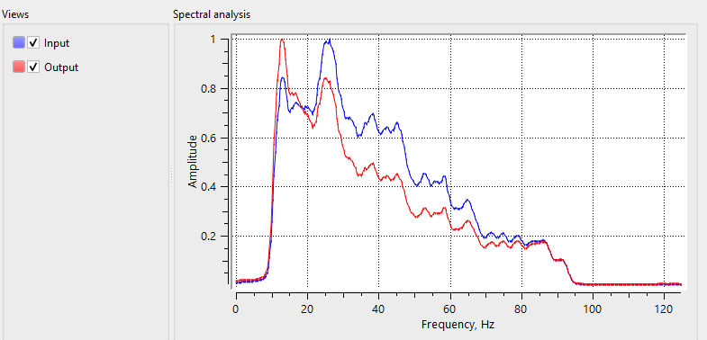
In this example, if we would like to compensate the lower frequencies, we can apply a 10% amplitude compensation at the lower frequency of 5 Hz. We can see the changes in the spectral analysis of both the input and output. Similarly, the user can work on with the different frequency amplitude pairs to compensate the geophone to get optimum results.
![]()
![]()
YouTube video lesson, click here to open [VIDEO IN PROCESS...]
![]()
![]()
Yilmaz. O., 1987, Seismic data processing: Society of Exploration Geophysicist
 * * * If you have any questions, please send an e-mail to: support@geomage.com * * *