Compensating the seismic data attenuation by using Q (Quality factor).

Theory

Seismic waves, especially high-frequencies, lose energy as they propagate through the Earth. This results in the recorded seismic data having lower resolution because the high-frequency components are diminished. So, Q compensation aims to restore those high frequencies that were lost, thereby improving the resolution of the seismic data.

The quality factor Q is a measure of the attenuation of seismic waves as they propagate through the Earth. Attenuation means the loss of energy. So higher Q means less attenuation, meaning the material is more elastic and the waves don't lose much energy. Lower Q means more attenuation, so the material is more inelastic, causing more energy loss.

Q = 2{\pi}\left ( \frac{E}{{\delta}E} \right )

Q  - Quality factor

          \frac{{\delta}E}{E}  -  fraction of energy lost per cycle

Earth acts as a filter that attenuates certain frequencies then Q compensation would apply the inverse of that filter to boost the affected frequencies. However, this must be done carefully because amplifying high frequencies can also amplify noise. Inverse Q filtering method involves in estimating the Q factor along the wave propagation path and then applying a gain to compensate for the attenuation.

Q compensation can be time-variant. Since attenuation increases with travel time, the compensation needs to be more aggressive for deeper reflections. since the waves travel deeper into the surface experience more attenuation. The main objective of the Q compensation is to enhance the resolution of the seismic data, recovering of the higher frequencies due to attenuation, better delineation of thin layers, and improved temporal resolution. Also, the wavelet should be corrected for the phase distortions caused by attenuation.

Some of the Q estimating methods include analyzing the amplitude decay with time or frequency content changes over time. If the Q model is inaccurate, the compensation might not work well or could introduce artifacts.

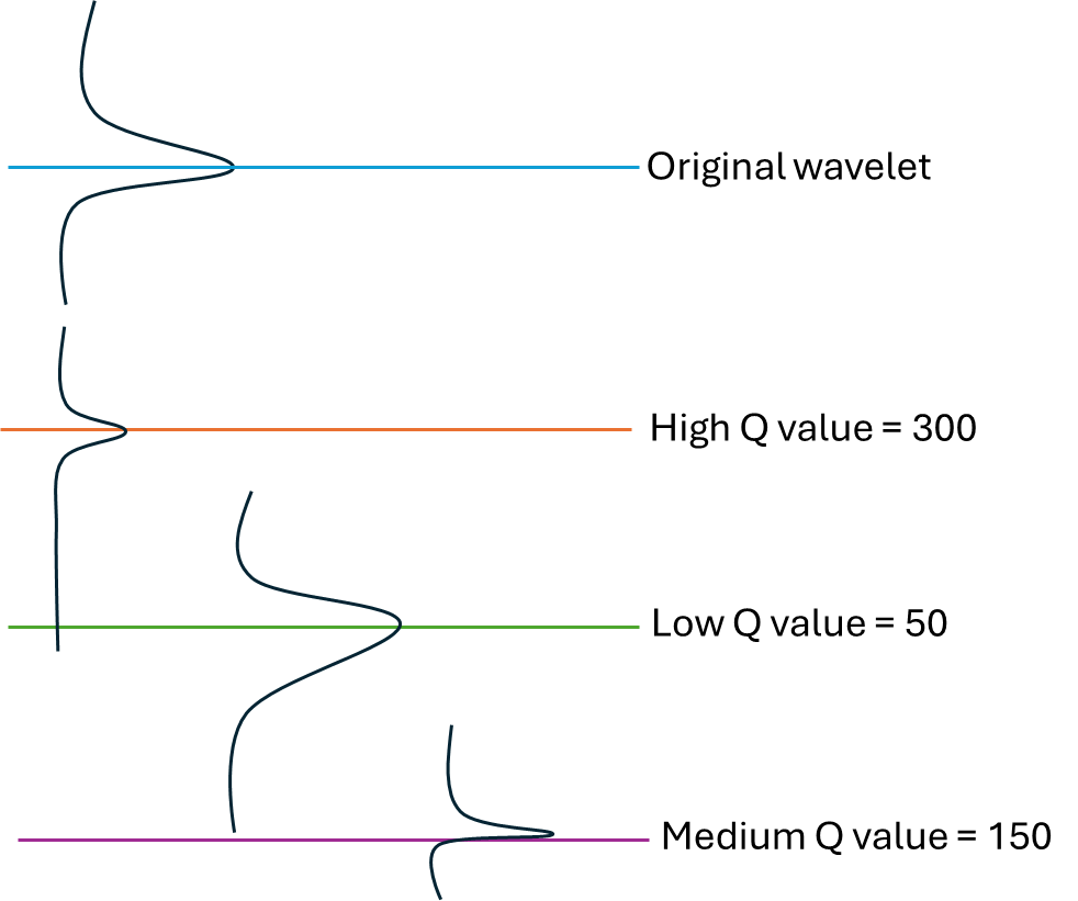
Higher Q value indicates that energy loss is minimal which translates to smaller amplitude peak as we can observe in the above image. With lower Q value, the wavelet broadens due to high energy loss. With respect to Medium Q value, the wavelet shape changes with mixed phase.

Input data

Input DataItem

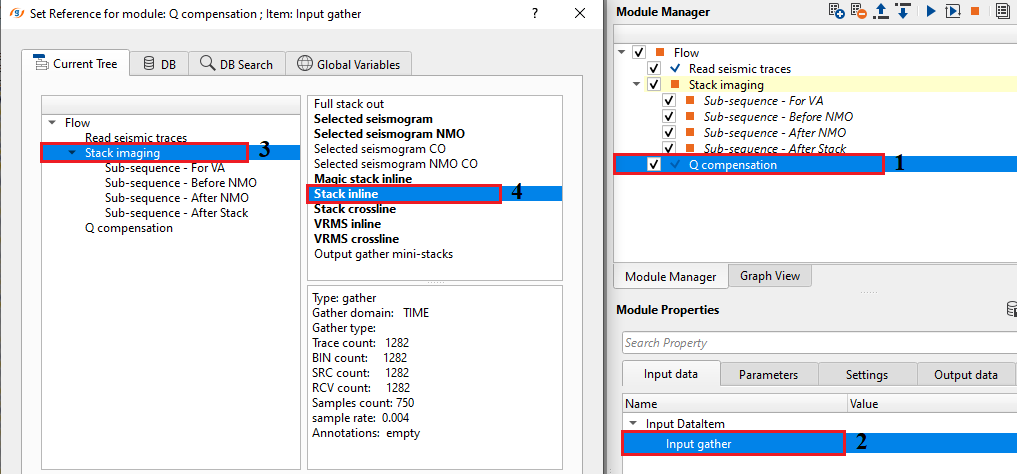
Input gather

connect/reference to the output volume/stack.

Parameters

Q-model type { Constant, Model, Time variant }

Choose the type of Q model type from the drop down menu.

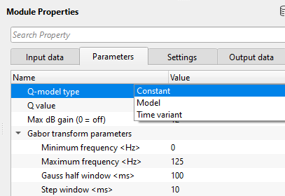
QModelType - Constant

By default, Constant option. Constant Q value is assumed when the frequency bandwidth doesn't change much even after propagating through the earth which means there is less energy loss. In general, seismic frequency range (say ~ 10 to 100 Hz) Quality factor (Q) doesn't vary much and stays stable.

Q value

Provide a constant Q value. By default, 120.

QModelType - Model

Provide the Q models generated from the Estimate Q factor modules. These models are helpful in compensating the energy attenuation by utilizing the combination of Q model, Q gain model & RMS velocity model.

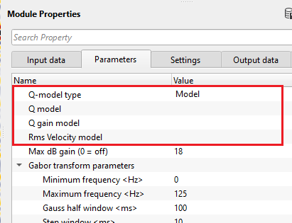
Q model

This is the estimated Q model generated from Estimate Q factor module. This Q model describes the spatial (horizontal) and temporal (vertical) variations of the Quality factor (Q) in the sub surface. A good Q model compensates the loss of energy properly however a poor Q model may result in artifacts.

Q gain model

This model represents how much gain is applied to seismic signal/wavelet at different times and frequencies to restore the lost energy due to attenuation. It calculates how much gain is required to compensate the seismic signal. This model is dependent on the frequency as we know that the higher frequencies attenuate more than the lower frequencies. Also, it is time variant as the attenuation happens differently at different times and gain increases with travel time.

Amplitude decay due to attenuation can be expressed as

              A(t,f)=A0​(f) e−πft/Q

A(t,f) - Amplitude at time t and frequency f

A0​(f) - Initial amplitude

Q - Quality factor

Q Gain model applies the inverse of this amplitude decay to compensate the lost amplitudes.

G(t,f)=eπft​/Q

G (t,f) - Gain at time t and frequency f

Q - Quality factor

This Q gain model requires the initial Q model and RMS velocity model. By using these two models, it calculates the gain function or Gain model for Q compensation.

Rms Velocity model

RMS velocity model is used to calculate the travel times. As we know, attenuation increases with the travel times and depth. So travel times are crucial for proper Q computation and compensation.

QModelType - Time variant

In this Q model, it considers the seismic signal attenuation with respect to change in time and/or depth. As the seismic signal propagates through the earth, the higher frequencies attenuate with increase in travel time. Whereas in case of the Constant Q model, it assumes that the attenuation is minimal and won't change through the sub-subsurface. Time variant Q model considers the sub-surface geological changes and compensates according to the lithology.

Q = Q(t)

Q(t) - Quality factor at time.

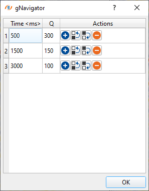
Time-Q function

Provide the Q values at different travel times.

Max dB gain (0 = off)

This parameter controls the under or over compensation of the Quality factor (Q). By default 18. Q compensation should not be over or under compensated. Over compensation may leads to noise boost, introducing artifacts.

Gabor transform parameters

Gabor transform is a time - frequency analysis technique which decomposes the seismic signal into frequency components with varying times. It is a kind of Fast Fourier Transform, where it divides the seismic trace/signal into small time windows and do the fast fourier transform within the window and move to the next window.

Minimum frequency

specify the minimum frequency which needs to be considered.

Maximum frequency

specify the maximum frequency

Gauss half window

provide the Gaussian window size where the seismic trace is analyzed.

Step window

provide the window step size.

Advanced

Reference frequency

Provide the reference frequency that needs to be compensated. This is a key parameter. It defines the frequency at which no amplitude and phase compensation is applied. All other frequencies are compensated relative to this frequency.

Q filtering { Modeling, Compensation }

Select the type of Q filtering from the drop down menu. Q Modeling generates the Q filter model for QC purpose whereas Q compensation option compensates the amplitudes decay.

Compensate amplitude

By default, TRUE (Checked). It will compensate the amplitude.

Compensate phase

By default, TRUE (Checked). Due to attenuation, phase of the seismic signal also changes. This needs to be compensated.

Preserve time gain

By default, TRUE. This option preserves the original time gain of the seismic signal.

Prewhitening (boost limit)

By default, 0.1. This is % white noise added to the signal to stabilize the output.

Settings

Auto-connection - By default, TRUE(Checked).It will automatically connects to the next module. To avoid auto-connect, the user should uncheck this option.

Bad data values option { Fix, Notify, Continue } - This is applicable whenever there is a bad value or NaN (Not a Number) in the data. By default, Notify. While testing, it is good to opt as Notify option. Once we understand the root cause of it, the user can either choose the option Fix or Continue. In this way, the job won't stop/fail during the production.

Notify - It will notify the issue if there are any bad values or NaN. This will halt the workflow execution.

Fix - It will fix the bad values and continue executing the workflow.

Continue - This option will continue the execution of the workflow however if there are any bad values or NaN, it won't fix it.

Calculate difference - This option creates the difference display gather between input and output gathers. By default Unchecked. To create a difference, check the option.

Number of threads - One less than total no of nodes/threads to execute a job in multi-thread mode. Limit number of threads on main machine.

Skip - By default, FALSE(Unchecked). This option helps to bypass the module from the workflow.

Output data

Output DataItem

Output gather

Generates the Q compensated output stack/volume.

Gather of difference

Generates the difference between the input stack/volume vs output stack/volume.

Information

There is no information available for this module so the user can ignore it.

Examples

In this example workflow, we are showing how the Q compensation works on a stack.

Connect/reference the stack section from Stack Imaging module to the Q compensation Input gather.

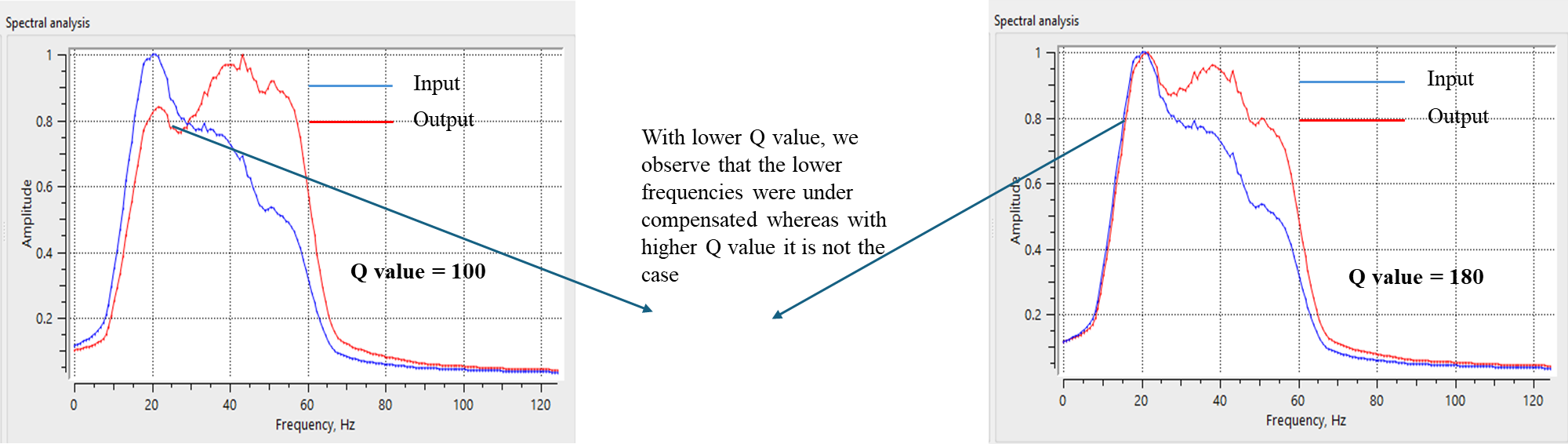
In the parameters, we are working on a Constant Q value. Test different Q values and QC the spectrum before and after Q compensation to provide the right/optimum Q value.

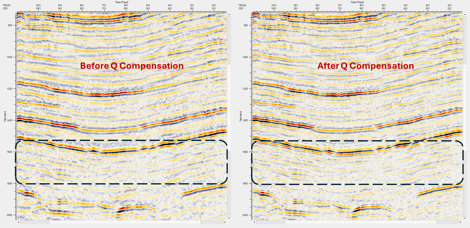
With a constant Q value of 180, we can see that the higher frequencies (dotted rectangles) are compensated. Reflections are clearly visible and the overall signal to noise is also improved.

Similarly, the user can test the other two methods i.e., Q model with Gain model along with RMS velocity model and Time - variant Q compensation.

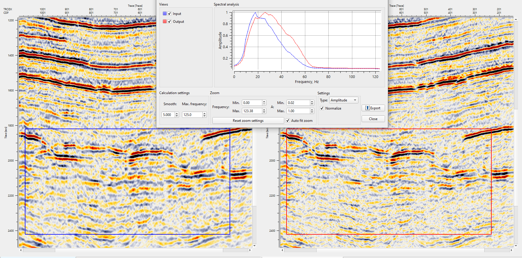
In this below example, we are showing a time variant Q compensation. The parameters for the time variant as

As we know that the attenuation of energy is less in the shallower part compared to the deeper part of the sub-surface. Higher frequencies attenuation is more in deeper part of the sub-surface which means lower Q value. In the below spectrum, amplitude is boosted the higher frequencies while keeping the amplitudes of the lower frequency range same.  

Actions

There are no action items available for this module so the user can ignore it.

Video lesson

YouTube video lesson, click here to open [VIDEO IN PROCESS...]

Related articles

Yilmaz. O., 1987, Seismic data processing: Society of Exploration Geophysicist

Sheriff, R. E., Geldart, L. P., (1995), 2nd Edition. Exploration Seismology. Cambridge University Press.

* * *   If you have any questions, please send an e-mail to: support@geomage.com  * * *