![]()
![]()
Fast Median Filtering is a non-linear filtering technique used in seismic data processing to suppress impulsive noise and spikes while preserving edges and reflection continuity. Instead of averaging samples (like mean filters), it replaces each sample with the median value from a local neighborhood, making it robust against outliers.
The module uses a computationally efficient histogram-based sliding-window algorithm. Rather than re-sorting all samples in the window from scratch at every step, it maintains a running amplitude histogram and updates only the samples that enter or leave the window as it slides across the gather. This makes the filter suitable for large datasets where a naive median sort would be too slow. The filter processes all traces in the gather in a serpentine (boustrophedon) scan pattern, updating the histogram incrementally as it moves.
Apply this module to pre-stack gathers before velocity analysis, NMO, or stacking to remove impulsive noise that would otherwise degrade semblance or stack quality. On post-stack data, it improves lateral reflector continuity without blurring reflection boundaries as aggressively as mean filters. Use it as an alternative to spike-detection-based despike modules when you prefer a statistical (median) replacement rather than interpolation from neighbours.
![]() Use smaller windows for pre-stack data (to avoid smearing moveout) and slightly larger windows for post-stack data.
Use smaller windows for pre-stack data (to avoid smearing moveout) and slightly larger windows for post-stack data.
How it works?
•A moving 2D window slides across the data (time × trace or inline × crossline).
•All samples inside the window are collected.
•The median (middle value when sorted) is computed.
•The center sample is replaced by this median (or compared against it, depending on implementation).
When to use it?
Pre-stack
•Remove spikes, bad traces, random impulsive noise
•Clean gathers before velocity analysis, NMO, or stack
•Preserve moveout trends better than mean filters
Post-stack
•Suppress residual random noise
•Improve lateral continuity of reflectors
•Edge-preserving smoothing prior to interpretation
![]()
![]()
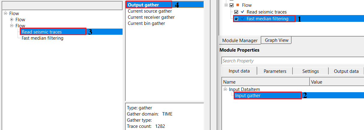
Input DataItem
Input gather - provide output gather (this could be pre or post-stack).
Connect any pre-stack or post-stack seismic gather to this input. The module accepts both common-midpoint (CMP) gathers with moveout and stacked time-domain sections. The output gather will have the same dimensions, sample interval, and header values as the input — only the amplitude values are replaced by their median-filtered counterparts.
![]()
![]()
Window X - Defines the horizontal window size (number of traces, inlines, or crosslines). It controls later smoothing. When the user uses large X values, it will suppress stronger noise however it is having a higher risk of smearing small features/events. By default, 10.
This is a half-width — the filter window extends Window X traces to each side of the current trace, so the total lateral span is (2 × Window X + 1) traces. Default is 10, meaning 21 traces are included in the window. Valid range: 0 to 1,000,000. Set to 0 to apply no lateral smoothing (time-only filtering). For pre-stack gathers, keep this value small (3–5) to avoid averaging across moveout trends. For post-stack data, values of 5–15 are typical for effective noise suppression. Larger values increase the computational cost only slightly because the algorithm uses an incremental histogram update rather than a full sort.
Window Y - Defines the vertical window size (number of samples or time/depth). It controls vertical smoothing. With larger Y values, it removes short period noise but distort thin beds. Attention must be paid. For both pre and post stack data, it is recommended to use smaller numbers. By default, 10.
This is also a half-width in samples. The window extends Window Y samples above and below the current sample, giving a total of (2 × Window Y + 1) samples in the vertical direction. Default is 10, meaning 21 samples in the window. Valid range: 0 to 1,000,000. A large vertical window will average over multiple reflection events and can blur thin-bed responses — keep it proportional to the dominant noise period you want to remove. If you are filtering with a 4 ms sample interval, a Window Y of 5 (covering 40 ms) is often a safe starting point. Set to 0 to disable vertical smoothing.
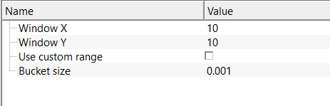
Use custom range - Limits the amplitude range considered during median calculation. Prevents extreme spikes from dominating the median and stabilizes filtering when data contain outliers or clipping. By default, FALSE.
When this option is disabled (the default), the module automatically scans the input gather to determine its actual minimum and maximum amplitude values, which are then used to define the histogram range. Enable this option when the automatic range detection is unreliable — for example, when the data contain extreme outlier amplitudes (dead traces clipped to a large constant, navigation artifacts, or recording equipment errors) that would cause the histogram to be sparsely populated over the true signal range, degrading the accuracy of the median estimate.
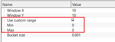
Use custom range - true - if this option is checked, provide the minimum and maximum amplitude values.
Min - provide the lower amplitude bound. By default, 0.
Set this to the expected minimum amplitude in your data (typically a large negative number for seismic data scaled to floating-point amplitudes, such as -10000 or -1.0 for normalized data). Amplitude values in the histogram that fall below this bound are clamped to the lowest histogram bucket rather than being excluded from the median calculation.
Max - provide the higher amplitude bound. By default, 0.
Set this to the expected maximum amplitude in your data. Together with Min, this defines the total amplitude range that the internal histogram spans. The number of histogram bins is (Max - Min) / Bucket size. Make sure Max is strictly greater than Min and that your signal amplitudes actually fall within this range. Values outside the range are clamped to the nearest boundary bucket and will still contribute to the median calculation, but their exact amplitude is no longer represented accurately.
Bucket size - Controls how data values are grouped internally to speed up median computation. Advantage of having larger bucket size is that faster processing, lower amplitude precision. On the contrary, smaller bucket size gives higher precision but slightly slower in execution. Use a bucket size small enough to preserve amplitude resolution but large enough for acceptable speed on big datasets. By default, 0.001
The bucket size is the amplitude width of each bin in the internal histogram. The total number of histogram bins equals the amplitude range divided by the bucket size: bins = (Max - Min) / Bucket size. A smaller bucket size yields more bins, giving a more precise approximation of the true median value, but requires more memory and slightly more time per update. A larger bucket size uses fewer bins and is faster but introduces a quantization error in the output amplitude equal to roughly half the bucket size. Default is 0.001. The minimum allowed value is 1e-6. For typical SEG-Y amplitude ranges (e.g., -10000 to +10000), a bucket size of 0.001 produces 20 million histogram bins — consider increasing the bucket size if your data has a very large amplitude range to keep memory usage reasonable.
![]()
![]()
Auto-connection - By default, TRUE(Checked).It will automatically connects to the next module. To avoid auto-connect, the user should uncheck this option.
Bad data values option { Fix, Notify, Continue } - This is applicable whenever there is a bad value or NaN (Not a Number) in the data. By default, Notify. While testing, it is good to opt as Notify option. Once we understand the root cause of it,the user can either choose the option Fix or Continue. In this way, the job won't stop/fail during the production.
Notify - It will notify the issue if there are any bad values or NaN. This will halt the workflow execution.
Fix - It will fix the bad values and continue executing the workflow.
Continue - This option will continue the execution of the workflow however if there are any bad values or NaN, it won't fix it.
Calculate difference - This option creates the difference display gather between input and output gathers. By default Unchecked. To create a difference, check the option.
Number of threads - One less than total no of nodes/threads to execute a job in multi-thread mode. Limit number of threads on main machine.
Skip - By default, FALSE(Unchecked). This option helps to bypass the module from the workflow.
![]()
![]()
Output DataItem
Output gather - generates output gather as a vista item. This output gather can be used for further processing.
The median-filtered seismic gather, ready for display or connection to the next processing module. All trace headers are preserved unchanged from the input gather. The amplitudes of each sample are replaced by their median-filtered values. This gather is visible in the Vista window for interactive quality control alongside the input gather.
Gather of difference - generates difference gather before and after applying median filtering.
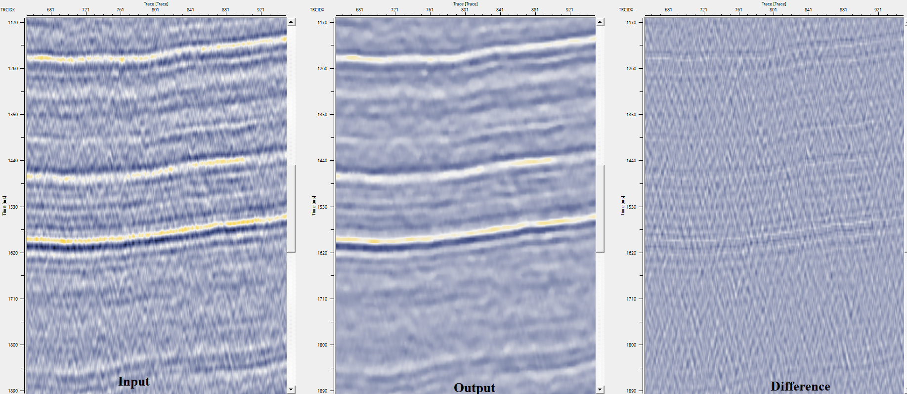
Available only when the Calculate difference option is enabled in the Settings section. This gather contains the sample-by-sample difference between the input and output (input minus output). It represents the noise that was removed by the filter. Inspect this gather to verify that the filter is attenuating noise rather than removing genuine reflection signal — the difference gather should look like random or incoherent noise, not like coherent reflections.
The example below demonstrates the use of Fast median filtering on a post-stack dataset to attenuate random noise.
![]()
![]()
In this example, we are reading a post stack dataset to attenuate/remove the random noise by using Median filtering.
![]()
![]()
There are no action items available for this module.
![]()
![]()
YouTube video lesson, click here to open [VIDEO IN PROCESS...]
![]()
![]()
Yilmaz. O., 1987, Seismic data processing: Society of Exploration Geophysicist
 * * * If you have any questions, please send an e-mail to: support@geomage.com * * *