Creating a Vibroseis sweep with user defined parameters
Description
The Create sweep module generates a synthetic Vibroseis pilot sweep signal from user-defined frequency, timing, and taper parameters. It is used in Vibroseis data processing workflows to produce a reference sweep for cross-correlation (Vibroseis deconvolution), simulation studies, or operator design. The module supports four sweep frequency sweep rate profiles and two amplitude taper shapes, giving full control over the sweep waveform characteristics.
The module outputs two gather items: one containing each individual harmonic trace plus a summed trace, and a second containing only the final composite sweep signal. Use the composite output as the pilot sweep for subsequent Vibroseis correlation or deblending steps.
What Is a Vibroseis Sweep?
A Vibroseis sweep is a controlled sinusoidal signal whose instantaneous frequency changes continuously from a low start frequency to a high end frequency (or vice versa) over the duration of the sweep. The vibrator truck injects this signal into the ground. The recorded seismic data is then cross-correlated with the known pilot sweep to produce a zero-phase or minimum-phase correlated record equivalent to an impulsive source record. The sweep shape, frequency range, duration, and taper directly determine the bandwidth and signal-to-noise quality of the correlated data.
The sweep timing is defined by four time markers: T1 (sweep start), T2 (end of leading taper), T3 (start of trailing taper), and T4 (sweep end). Between T1 and T2 the amplitude ramps up; from T2 to T3 the amplitude is at full strength; and from T3 to T4 the amplitude ramps back down to zero. This tapering reduces spectral leakage and transient effects at the ends of the sweep.
Harmonics arise from non-linear distortion in the vibrator mechanism. This module can simulate multiple harmonic orders simultaneously, allowing you to study or design deblending strategies that account for harmonic interference.
There are input data requirements for this module. Everything should mention in the Parameters tab.
Parameters
Number of harmonics - define the number of harmonics. If more than 1 harmonic is added then the sweep energy will be more complex. Each additional harmonics add a sinusoidal component and increases the fundamental frequency.
Set how many harmonic orders to include in the sweep model. The fundamental sweep (first harmonic) is always generated. Setting this value to 2 adds a second-order harmonic trace at twice the instantaneous frequency, setting it to 3 adds a third-order harmonic, and so on. The "Sweep with harmonics" output gather will contain one trace per harmonic plus a summed trace combining all harmonics. The "Modeled sweep signal" output always contains only the summed composite signal.
Default: 1 (fundamental harmonic only). For most standard Vibroseis processing workflows, a value of 1 is appropriate. Use higher values (typically 2 or 3) when modelling harmonic distortion effects or designing harmonic deblending operators.
Start Frequency Fr1 - specify the starting frequency of the sweep. By default, 1.
The low-frequency end of the sweep band in Hz. The instantaneous frequency of the generated sweep begins at this value at time T1 and increases toward the End Frequency over the sweep duration. Choose a value that matches the low-frequency capability of the vibrator and the target geological bandwidth. Typical field sweeps start between 6 Hz and 12 Hz, though modelling sweeps may use lower values.
Default: 1 Hz. Units: Hz.
End Frequency Fr2 - specify the ending frequency of the sweep. By default, 5.
The high-frequency end of the sweep band in Hz. The instantaneous frequency reaches this value at time T4. The difference between Start Frequency and End Frequency defines the bandwidth of the generated sweep. A wider bandwidth produces a shorter autocorrelation wavelet (Klauder wavelet) after correlation, which improves temporal resolution. Ensure this value does not exceed the Nyquist frequency derived from the Sweep dt (Nyquist = 0.5 / dt in Hz).
Default: 5 Hz. Units: Hz.
Sweep type { Linear, DB/Hz, DB/oct, T-power } - select what kind of sweep to create. By default, Linear.
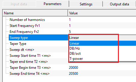
Controls how the instantaneous frequency changes with time across the sweep duration. This setting determines the spectral energy distribution of the sweep and, consequently, of the correlated Vibroseis data. Four options are available:
Linear — Frequency increases at a constant rate from Fr1 to Fr2 over the sweep duration. This is the most widely used sweep type in the field. It produces a flat amplitude spectrum (equal energy per Hz) after autocorrelation, making it the standard choice for most Vibroseis acquisition programs.
DB/Hz — The sweep rate is adjusted so that the output spectrum amplitude changes by a specified number of decibels per hertz. Use this type when you need to boost or suppress specific frequency ranges by a fixed dB/Hz amount. The Decibels per hertz parameter becomes active when this type is selected.
DB/oct — The spectral amplitude changes by a specified number of decibels per octave. This is a standard way to pre-whiten or tilt the spectrum of a sweep to compensate for frequency-dependent earth attenuation or vibrator output characteristics. The Decibels per octave parameter becomes active when this type is selected. Note that a value of -6 dB/oct is treated as -5.999 internally to avoid a singularity.
T-power — The instantaneous frequency follows a power-law function of time. This allows non-linear time-frequency relationships where the sweep dwells longer at lower or higher frequencies depending on the power exponent. The Power of time parameter becomes active when this type is selected. A value of 1.0 approximates a linear sweep; values greater than 1 increase dwell time at low frequencies.
Default: Linear.
Decibels per hertz - the spectral slope in dB/Hz applied when Sweep type is set to DB/Hz. Positive values amplify high frequencies relative to low frequencies; negative values do the opposite.
This parameter is visible only when Sweep type is set to DB/Hz. It specifies the rate of amplitude change across frequency, in decibels per hertz. Use this to shape the sweep spectrum to compensate for frequency-dependent effects in the acquisition system or to pre-condition the sweep energy for a desired post-correlation result.
Default: 0 (no slope; equivalent to a flat spectrum). Units: dB/Hz.
Decibels per octave - the spectral slope in dB/octave applied when Sweep type is set to DB/oct. This controls how much the sweep amplitude changes for each doubling of frequency.
This parameter is visible only when Sweep type is set to DB/oct. A value of +6 dB/oct means the amplitude doubles for each octave increase in frequency (boosting high frequencies). A value of -6 dB/oct halves the amplitude per octave (attenuating high frequencies, which mimics an earth-like attenuation curve). Avoid setting exactly -6; the value -5.999 is used internally if you do.
Default: 0 (no slope). Units: dB/octave.
Power of time - the exponent that controls the non-linearity of the frequency-versus-time relationship when Sweep type is set to T-power.
This parameter is visible only when Sweep type is set to T-power. The instantaneous frequency at time t within the sweep is proportional to t raised to this power. Setting the exponent to 0 produces a constant-frequency (non-sweeping) signal. A value of 1 gives a linear sweep behaviour. Values between 0 and 1 cause the sweep to spend more time at higher frequencies; values greater than 1 cause more dwell time at lower frequencies.
Default: 0. Units: dimensionless.
Taper Type { Cos2, Linear } - these tapers are helpful in smoothing of the sweep at the start and end by avoiding any jumps. By default, Cos2.
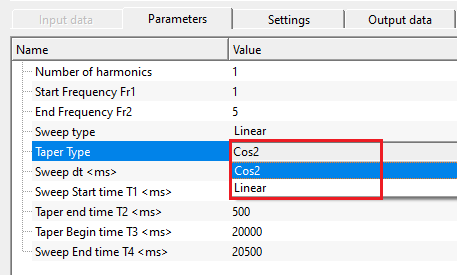
Controls the shape of the amplitude envelope applied at the beginning and end of the sweep (the lead-in taper from T1 to T2 and the lead-out taper from T3 to T4). The taper prevents abrupt amplitude steps that would introduce broadband spectral artefacts and improve the correlated Klauder wavelet shape. Two options are available:
Cos2 — Applies a squared-cosine (Hann-like) ramp. The amplitude envelope is proportional to sin²(x) during the lead-in and cos²(x) during the lead-out. This is the most common choice because the smooth, rounded shape minimises spectral leakage and produces a clean Klauder wavelet after autocorrelation.
Linear — Applies a straight-line ramp from zero amplitude to full amplitude during the lead-in, and from full amplitude back to zero during the lead-out. This is simpler but has slightly more leakage than the Cos2 shape. It may be appropriate when reproducing specific legacy field sweep designs.
Default: Cos2.
Sweep dt - this is the sampling interval of the sweep. Specify the sampling interval in ms. By default, 2 ms.
The time sampling interval of the generated sweep signal, in seconds. This controls the digitisation rate of the output traces and determines the Nyquist frequency (maximum representable frequency = 0.5 / dt). For example, the default value of 0.002 s (2 ms) gives a Nyquist frequency of 250 Hz. Set this to match the sample interval of the seismic data that will be cross-correlated with this sweep. If the sweep End Frequency approaches or exceeds the Nyquist, aliasing artefacts will appear in the output.
Default: 0.002 s (2 ms). Units: seconds (s).
Sweep Start time T1 - this is the starting time of the sweep. At this time, amplitude of the sweep is zero. By default, 0
The time at which the sweep signal begins, in seconds. Before T1 the amplitude is zero. At T1 the lead-in taper starts ramping up from zero. For most applications this is set to 0 so the sweep starts at the beginning of the trace. A non-zero T1 can be used to add a silent pre-sweep period to the output trace.
Default: 0 s. Units: seconds (s). Must be less than or equal to T2.
Taper end time T2 - this is the initial taper end time. The amplitude between T1 & T2 gradually increases. By default, 500
The time at which the lead-in taper reaches full amplitude, in seconds. From T1 to T2 the amplitude ramps from zero up to its maximum value following the chosen Taper Type shape. From T2 to T3 the sweep amplitude is constant at its maximum (fully on). Longer T2 intervals provide a smoother, more gradual ramp-up but use more of the total sweep duration for the taper. In field acquisition, lead tapers are typically 100 ms to 500 ms long.
Default: 0.5 s (500 ms). Units: seconds (s). Must be greater than or equal to T1 and less than T3.
Taper Begin time T3 - this is the ending taper time. The amplitude between T3 & T4 gradually decreases. By default, 20000.
The time at which the lead-out taper begins, in seconds. From T3 to T4 the amplitude ramps from its maximum back down to zero following the chosen Taper Type shape. The interval between T2 and T3 is the full-amplitude portion of the sweep; the interval between T3 and T4 is the trailing ramp. Adjusting T3 controls the length of the trailing taper, which should match the field acquisition design.
Default: 20 s. Units: seconds (s). Must be less than T4.
Sweep End time T4 - this is the ending time of the sweep. At this time, amplitude of sweep is zero. By default, 20500.
The total length of the generated sweep trace in seconds. After T4 no samples are generated; the total number of output samples equals T4 divided by the Sweep dt. At T4 the amplitude has returned to zero following the trailing taper. This parameter effectively defines the total sweep record length. For a typical 20-second field sweep with 0.5-second lead and trail tapers, set T4 to 20.5 s (matching the default).
Default: 20.5 s. Units: seconds (s). Must be greater than T3.
Settings
Skip - By default, FALSE(Unchecked). This option helps to bypass the module from the workflow.
When enabled, the module is bypassed entirely and passes no output to downstream modules. Use this to temporarily disable sweep generation without removing the module from the workflow. Useful when testing different workflow configurations.
Output data
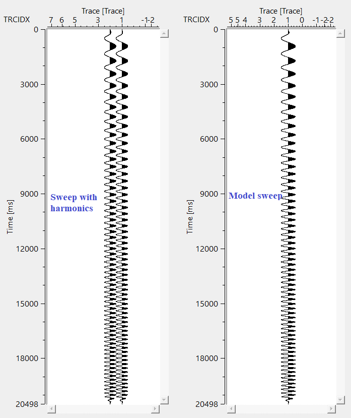
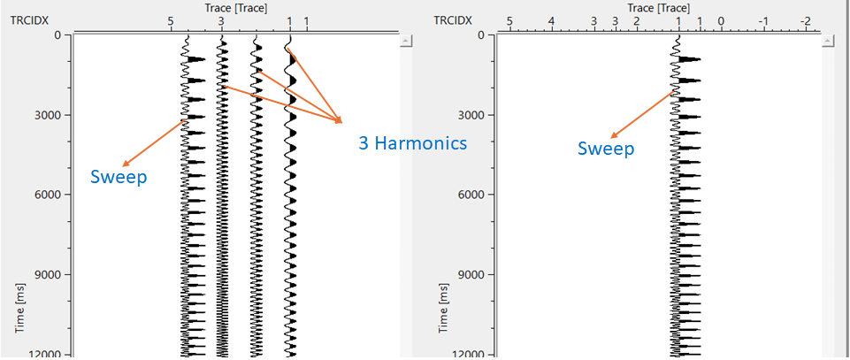
Sweep with harmonics - generates and outputs sweep with harmonics. If the number of harmonics are three then there will be 4 traces (1 sweep + 3 harmonics)
A multi-trace gather where each trace represents one harmonic order of the generated sweep, plus a final trace that is the sum of all harmonic traces. For example, if Number of harmonics is set to 3, the output gather contains 4 traces: the fundamental (first harmonic), the second harmonic, the third harmonic, and the composite summed trace. This output is useful for inspecting the contribution of each harmonic individually or for designing harmonic-specific deblending operators.
Modeled sweep signal - this is the final generated sweep.
A single-trace gather containing the composite sweep signal — the sum of all harmonic components. This is the primary pilot sweep to use for cross-correlation with Vibroseis field records, for Vibroseis deconvolution, or for the deblending operator design workflow. It contains the same composite trace as the last trace of the "Sweep with harmonics" output.
There is no information available for this module.
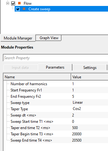
Example
In this example workflow, we generate a sweep with the default parameters.
Actions
There are no action items available for this module so the user can ignore it.
References
![]()
![]()
Yilmaz. O., 1987, Seismic data processing: Society of Exploration Geophysicist