In this section, we are going to describe how to test and execute the DI work flow. For the example, we are using Teapot Dome 3D dataset. For the study, we have taken the preprocessed gathers and velocity(migration velocities) as input(s). We know that the input data consists of both reflections and diffraction energy however the diffractions energy is so small that we couldn't able to see them on the shot gather. To overcome that, we generate the synthetic diffractions. The approach is outlined below.
Phase -1:
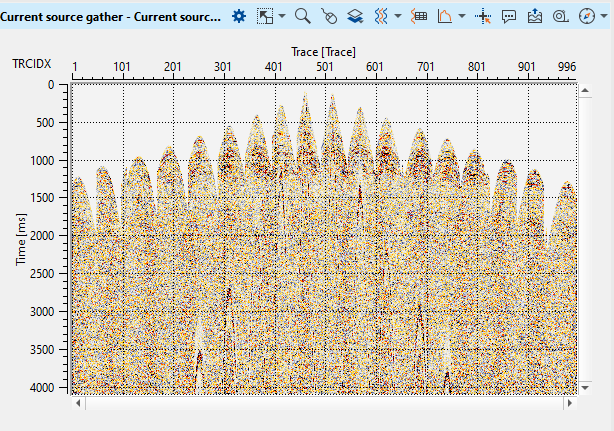
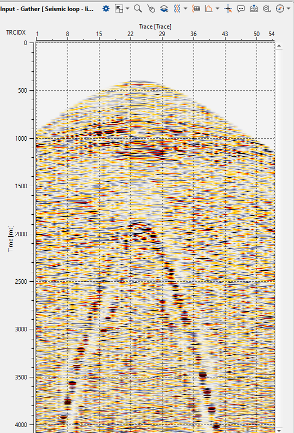
1. From the input gathers, we select a single shot gather (One Receiver Line and corresponding Receiver SP) from the volume and save it.
2. Read this single shot gather. The objective of this single shot gather exercise is to create synthetic diffractions with the matching amplitudes of the input shot gather and superimpose the diffractions.
3. Create Synthetic diffractions using Frac modelling module. The output from the Frac modelling is the combination of reflection and diffraction energies.
4. Now read the shot gather (reflections+ diffractions) and shift the data to DATUM. In case the data is marine, the user can ignore this step since the DATUM is referenced to MSL (Mean Sea Level).
5. Apply forward NMO correction to flatten the reflections.
6. Do some denoising by using Despike module if it is necessary.
7. Test and run Wave separation by gather (Local Plane Wave Detection/Decomposition (LPWD)) module to attenuate the reflection energy only and keep the diffractions.
8. Now do reverse NMO correction.
9. Shift the data back to Topography.
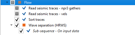
The above procedure is the testing phase where the user should test the parameters on any shot gather from the entire volume to check the parameters are good enough to run/execute on the entire volume. Prior to that, for a quick QC, we advised the user to run the module "Wave Separation (HRWS)" and execute only for one single shot to check the output. Once satisfied, run for the entire using the module "Wave Separation (HRWS)".
In the following section, we are going to show Phase 1 where we need to extract a single shot gather and attenuate the reflection energy.
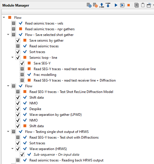
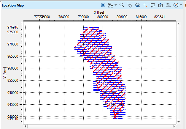
1. Select the shot gather from the location map of the "Read seismic traces" module.
2. From the selected shot gather, we will sort the data in RECEIVER_LINE & RECEIVER_SP order using "Sort traces" module and select single shot gather. In case the data is 2D, the user can sort the data in FFID-Channel or FFID-Offset order.
3. Save this selected shot gather using "Save SEG-Y" module and read back the shot gather using "Read SEG-Y traces" module.
4. Create the synthetic diffractions on the selected gather using "Frac modelling" module as shown below. More in detail about Frac modelling is covered at the end of this section
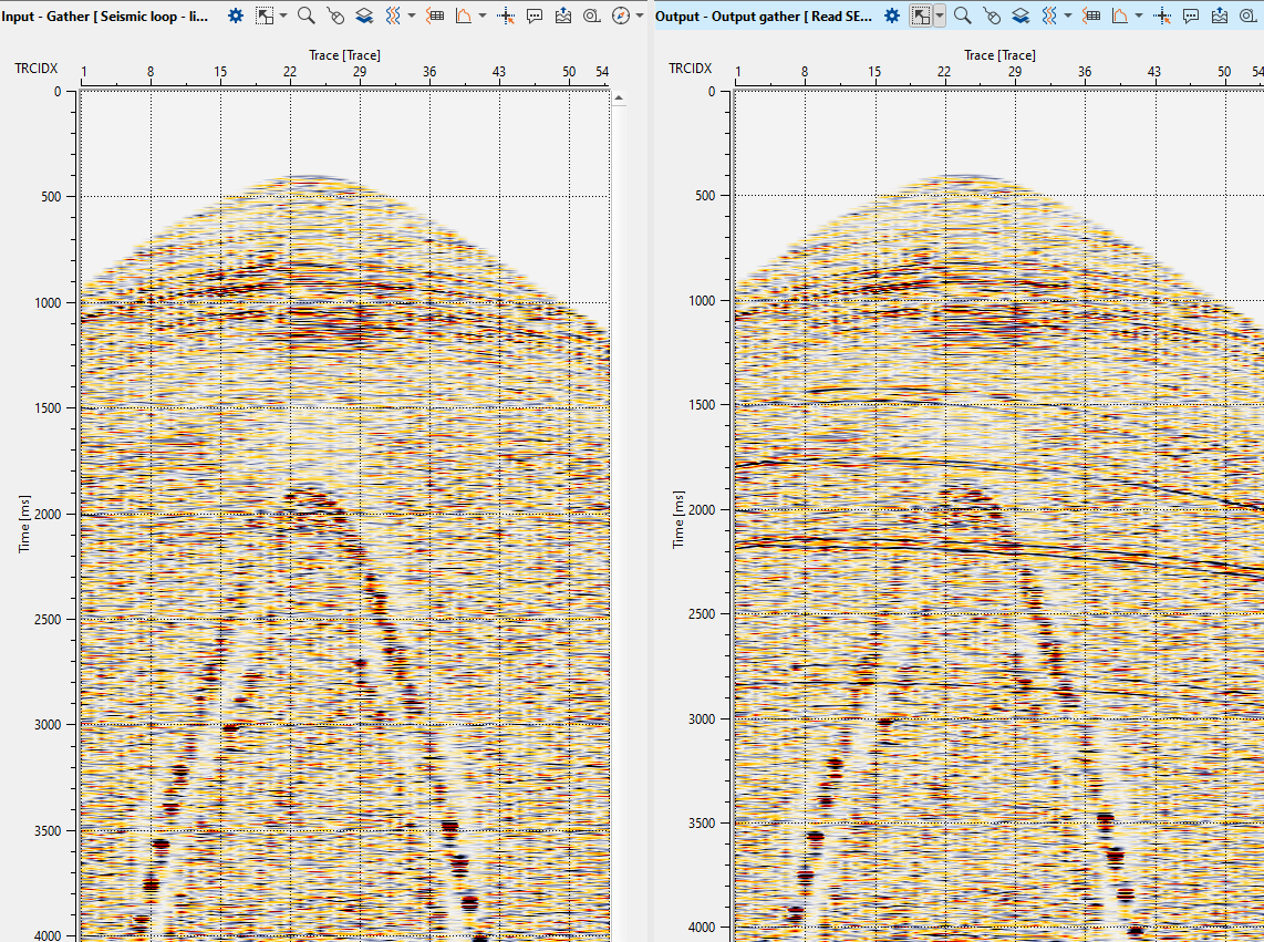
5. Once the shot gather is having both reflections and diffractions energy, we are ready to move to the next stage i.e. shift data to datum, NMO correction, Despike followed by Wave separation by gather (LPWD) as shown below.
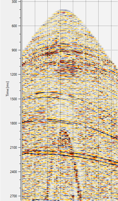
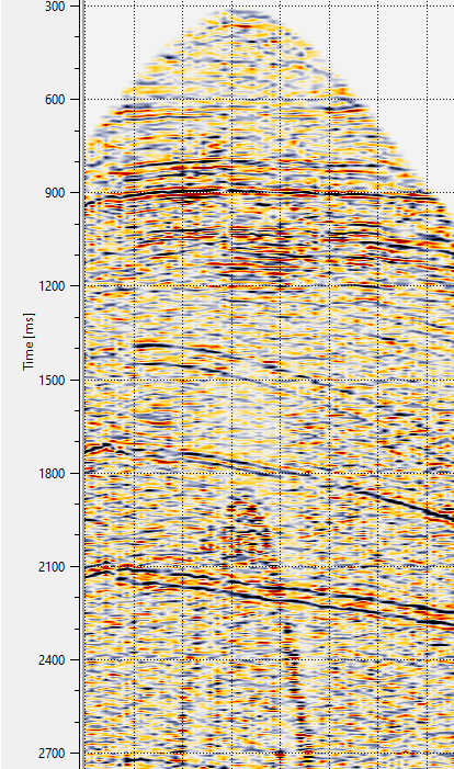
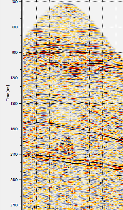
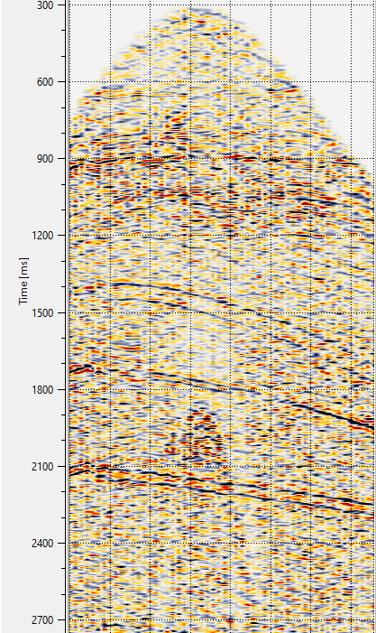
From the above images ( last image (left to right)), we can observe that we've successfully attenuated the reflection energy and kept the diffraction energy only. Similarly, the user should check the parameters at different locations on the location map to confirm that the parameters are good enough for the entire volume.
Prior to the full volume execution of HRWS module, it is advised to run on a single shot gather to see output.
Phase 2 :
From Phase-1, we got the reflection energy free data using Wave Separation (HRWS) module. Now we need to calculate the Diffraction Coherency & Energy attributes from the input data. Following is the procedure to get both the attributes.
1. Read input data (Diffractions energy only) using "Read seismic data"module. If necessary do the Binning 3D. Followed by sorting the data in INLINE-XLINE/OFFSET using Sort traces module.
2. Similarly read the velocity information (as per the velocity format). If it is in gather format, use "Read seismic traces" module. Please make sure that input data and velocity data should have same number of samples and sample interval. If necessary do the binning using "Binning 3D" module.
3. We need an input stack for output geometry information. So the user should read the stack using "Read seismic traces" module.
4. Run Engine - Diffraction imaging 2D/3D module to calculates the semblance of all diffraction energy of prestack seismic data and store it in a storage file.
5. Execute Imaging - Diffraction 2D/3D module to extract the Diffraction coherency and energy attributes. This module generates Fold & Semblance as attributes. The user should use these attributes information to generate the Diffraction Coherency and Diffraction Energy attributes.
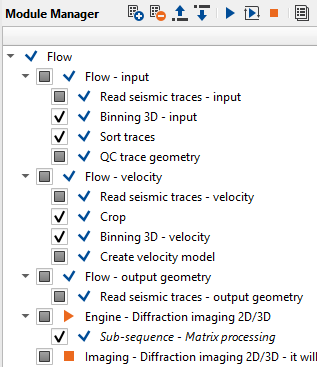
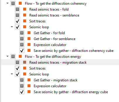
On the above images, on the left side image we have the initial workflow to read the seismic and velocity data. In Engine - Diffraction imaging 2D/3D, we calculates the semblance of the diffraction energy and stores in a file. This storage file will be input to the Imaging - Diffraction imaging 2D/3D module. It will generate the Fold & Semblance attributes.
On the right hand side workflow, we read the fold and semblance attributes and do the multiplication using the "Expression calculator" to generate the Diffraction Coherency. To generate the Diffraction Energy, we need to multiply the migration stack with itself using "Expression calculator" module.
Frac modelling
The objective of Frac modelling is to create synthetic diffraction energy and add this diffraction energy into the reflection data. You may think that why we need to do the model the diffractions. Well, the input data is having both reflection and diffraction energy however diffraction energy is dominated by the dominant reflection energy which we couldn't find. To attenuate all the reflection energy and keep only diffraction energy we should find a suitable parameters. For the same reason, we model the diffraction energy with the same characteristics of the input data (frequency, amplitude, wavelength etc) and try to attenuate all the reflection energy. These same parameters we apply later on the input data to have only Diffraction energy.
To get the synthetic diffractors,
1.Measure the frequency and wavelength of the input data (may be consider a single trace or full shot gather). For this, you can use Spectral analysis to measure the frequency. For measuring the wavelength, you can display the data in wiggle mode. These parameters needs to be provided in the WaveParams of Frac Modelling to match the frequency and wavelength of the synthetic diffractor with the input data.
2.In case the data is 3D, we should provide all the parameters however if the data is 2D, the user can test the Crossline step parameter.
a.Inline step - Provide the inline step size in creating the diffraction energy
b.Crossline step - Provide the cross line step size for creating the diffraction energy. In case of 2D data,
c.Each time – At what interval the next diffractor wave generated
d.First time – At what time, the diffractor should start
e.End time – Provide the End time to stop creating the diffractors below the defined end time
f.Amp value – To have more or less the same amplitude level of the input data (reflection energy).
g.AmpPow – This is in tandem with Amp value parameter.