Multiple Attenuation (SRME)

SRME is an acronym which can be elaborated as Surface Related Multiple Elimination or Estimation

The presence of multiples in the data will give a false information to the interpreters. To attenuate the multiples we need an algorithm which can predict the multiples from the input data and later subtract the multiples from input to get the multiple free data. It can be achieved in different ways.

1.Periodicity based

2.Move out based

Surface related multiples is predicted using auto-convolutions of input data. The predicted multiple energy is then adaptively subtracted from the input gathers.

Create a workflow 0100-srme

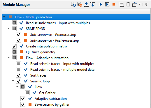
It is a two step process. First we predict the multiple from the input data. In the second part, we read the input data with both primaries and multiples followed by multiple predicted gathers. In this step, we do the adaptive subtraction to attenuate the multiples to get the multiple free data.

1. Read seismic traces

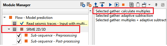
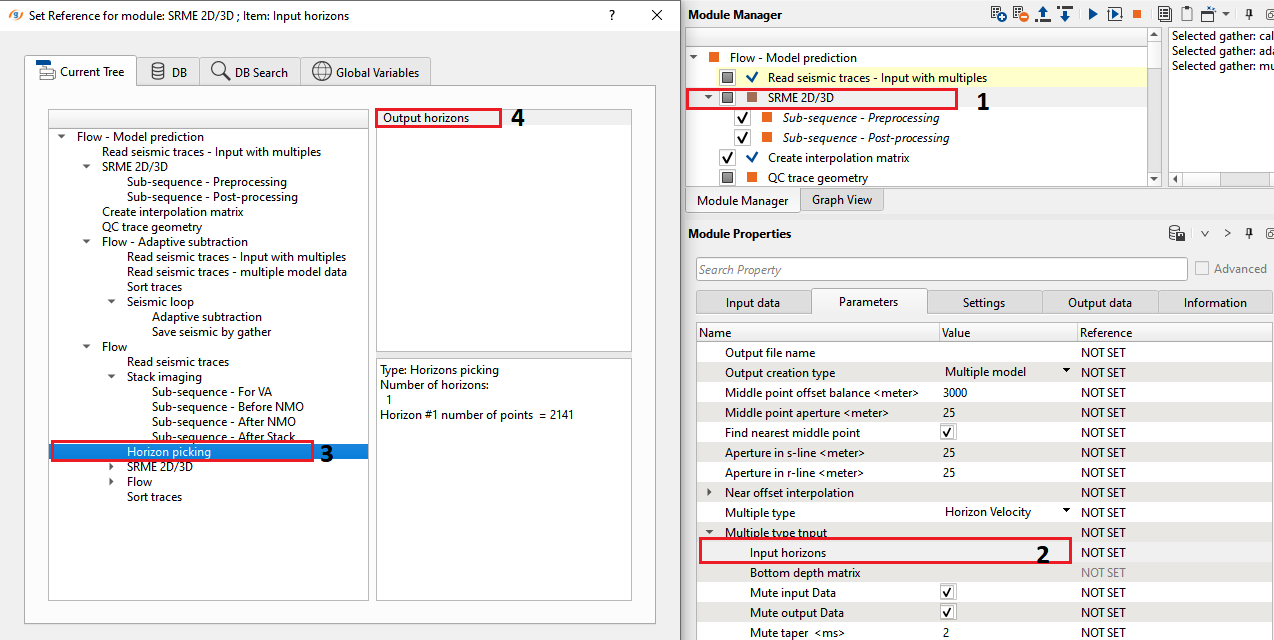
2. SRME 2D/3D

3. Create interpolation matrix

4. QC trace geometry

5. Read seismic traces

6. Read seismic traces

7. Sort traces

8. Seismic loop

9. Adaptive subtraction

10. Save seismic by gather

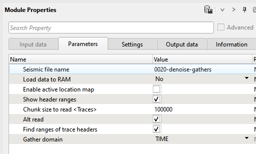
1) Read seismic traces loads seismic trace from the previous step, input file name is 0020-denoise-gatgers. Execute the module by double click on it or press on run button from the upper menu.

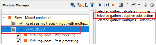
2) SRME 2D/3D This is the first stage of SRME. In this, we prepare the multiple model (check the input data has water bottom times, direct arrivals are muted etc. If the water bottom times are not available, the user can pick the horizon and get the times by using Create interpolation matrix module which explained in the following module).  

Make the necessary connections as show in the above image and test the parameters.

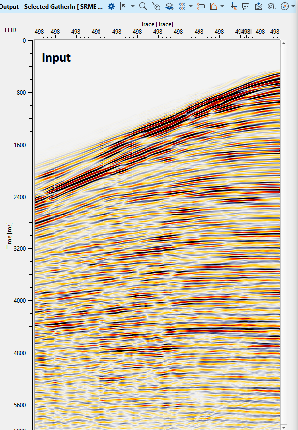
In order to predict the multiple model, first supply the input data. Launch the Vista all groups and select any shot from the location map ( Preferably the shots which are not close to the start of the line).

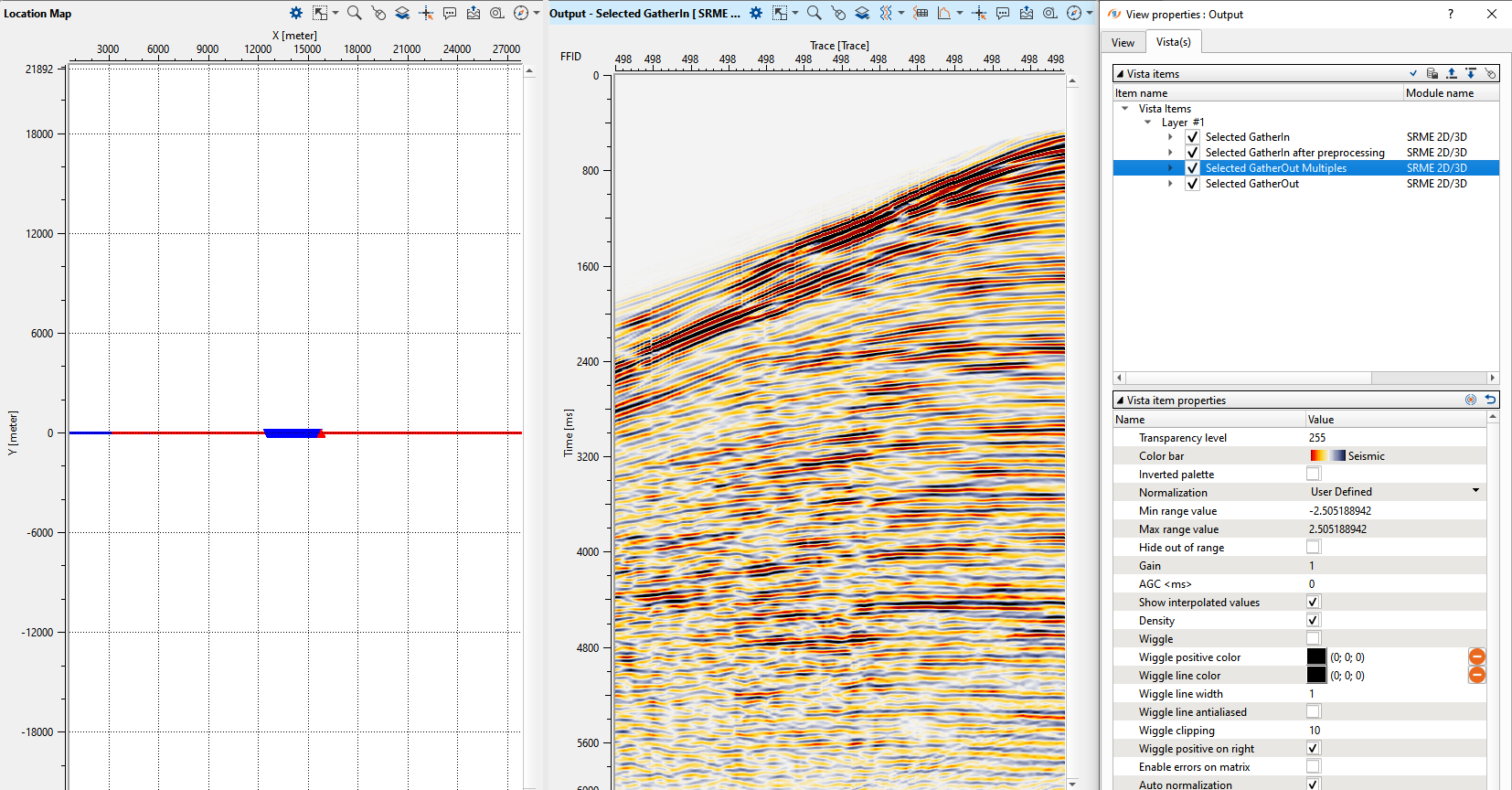
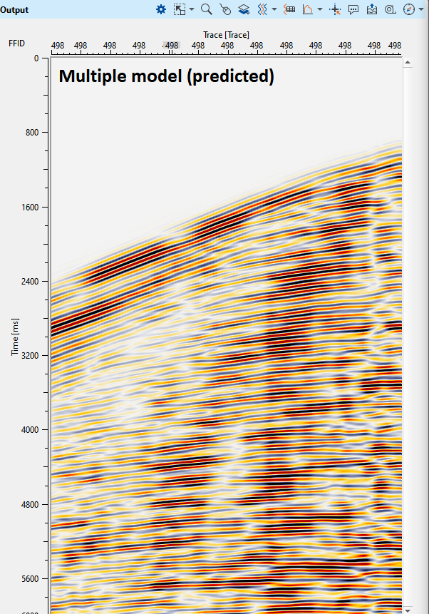
Once the shot is selected from the location map and it is displayed, now click the “Selected gather: calculate multiples” option in the action items menu which gives the predicted multiple for that particular shot.

Now turn on/off the "Selected gathers" and/or "Selected gathers out multiples" to check the predicted multiple by clicking on the Show properties icon of Output - Selected GatherIn [SRME 2D/3D] window.

Adjust the parameters and try at different shot location to see the predicted multiple model is satisfactory. Once the user satisfied with the predicted model, we can do the adaptive subtraction to see whether the predicted model is good enough to attenuate the multiples. The key part is not only the predicted multiple model but also the adaptive subtraction parameters to have a better multiple free data. Enough testing should be carried to before proceeding towards production workflow.

Now click on the “Selected gather: adaptive subtraction” which can adaptively subtract the multiples and gives you the multiple free data. This adaptive subtraction and the parameters of the adaptive subtraction is just for a visual inspection to QC the results however the user should adjust the parameters in the second part of the workflow where the Adaptive subtraction module has more parameters to work on with.

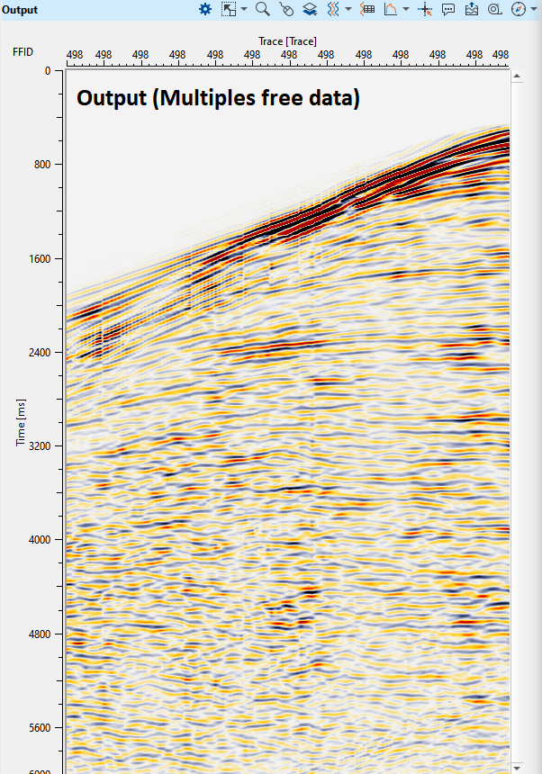
In the above image, we have shot before multiple attenuation and after multiple attenuation.

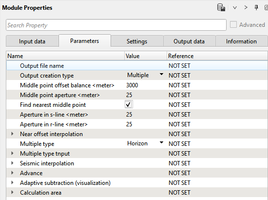
Output file name

Provide the predicted multiple model output file name

Output creation type

Select the output creation type from the drop down menu. By default it is "Multiple model"

Middle point offset balance

This is the differential distance between the source and receiver ray paths of the multiple model. For example, if the source and receiver combination having multiple (many) multiple ray paths then the distance between one of the ray path to the remaining ray paths should be equal or greater than this value if not these multiple ray paths are considered in calculating the multiple prediction model.

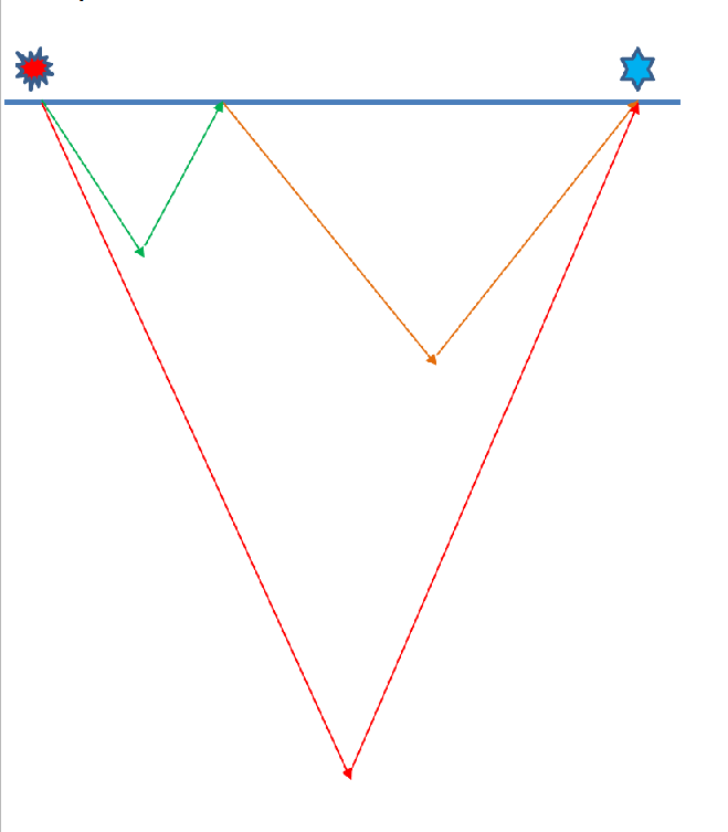
In the above image, we have source and receiver. Consider that we have 480 channels (receivers) and the receiver interval as 12.5 meters so the offset should be (480*12.5 = 6000 meters). The ray path distance from source to receiver (consider somewhere in receiver spread for easy understanding of the middle point offset calculation) is 3000 meters. Now we have double bounce (Green ray path and Brown ray path). If the distance between these ray paths are considered as 1000 meters and 2000 meters and difference is 1000 meters. Now if the user considers that a middle point offset is 600 meters then all the source and receiver combination ray paths falling within or above this offset range value are considered in calculating the multiple prediction model. In other sense, any Source-Receivers pair middle point offset falling below 600 meters were not considered in the multiple prediction.

Middle point aperture

The distance between the nearest source and receiver pair.

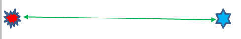
In the above, the distance between the source and 1st channel is 12.5 meters. If the user provides a value of 20 meters as a middle point aperture, it will search for the traces falling within this aperture and consider them in calculating the multiple model.

Find nearest middle point

By default False. If user checks the option then it automatically searches for the nearest middle point. In this instance the middle point aperture in the previous parameter will not be considered.

Aperture in s-line

Aperture in In Line direction for a searching all sources and receivers, which will be involved in the modeling of multiples for current trace

Aperture in r-line

In case of 3D, Aperture in Cross Line direction for a searching all sources and receivers, which will be involved in the modeling of multiples for current trace

Near offset interpolation

In case if there are any missing shots at the beginning of the line, then turn ON this option to do the interpolation for better predicting the multiple model.

Replacement velocity

Provide the near surface/replacement velocity or water velocity

Maximum distance to interpolate

Define the maximum distance for interpolation which is related to near offset interpolation

Step to interpolate

Define the interpolation step size. Usually the receive interval or shot point interval.

Multiple type

Select the type of multiples from the drop down menu. Depending on the selection , the user should provide the respective input information. For example, if the multiple type is selected as "Horizon velocity model" then they should provide the horizon information in the Multiple type input section.

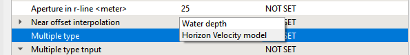
Water Depth: Multiple model prediction based on Source Water Depth values.

Horizon Velocity Model: You can pick the water bottom horizon using the Horizon picking module and provide the horizon information here.

Multiple type input

Input horizons

In case the multiple type is chosen as "Horizon velocity model" the we should provide the horizon.

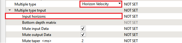
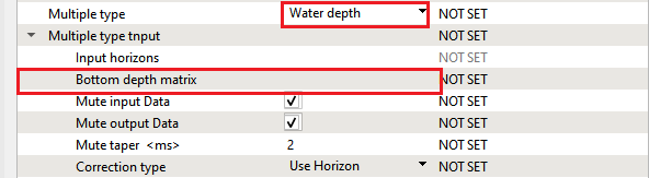
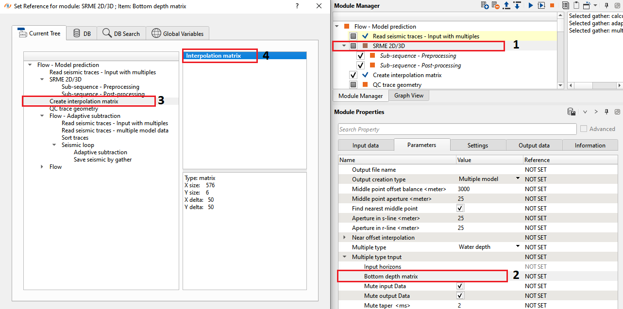
Bottom depth matrix

Connect to the Source Water Depth values. It can be created by using Create Interpolation Matrix module.Provide the depth matrix if the multiple type as "Water depth"

Mute input Data

By Default True. Its user choice. It’s advised to check your input data if you select this option as True to make sure you have all the input information and no primary data is muted..

Mute output Data

By Default True. Same as Mute Input Data. Check your final output data.

Mute taper

Provide the mute taper value to apply the mute the gather above provided taper value.

Correction type

Select the correction type. By default "Use horizon correction"

Seismic interpolation

Interpolate input traces

Prior to model prediction, user can to interpolate the input traces. By default it is set as False but user can select this option.

Trace multiplication factor

Define the trace interpolation (multiplication factor). For example, if shot interval is 25 m and receiver interval is 12.5 m and we want to interpolate every shot to make the shot interval is same as receiver interval to predict the multiple model more accurate.

Number of iterations

Define how many iterations are required to interpolate the input traces. Remember the more number of iterations the more run time it takes. 10 no of iterations is a good starting point.

Regularization type

Choose the regularization type from the available options. By default Laplasian.

We have 4 types of regularization in case if we have any missing traces or shots. Choose the appropriate one for the data regularization among the given one.

1. First derivative

2. Laplasian

3. FK

4. Radon

Depending on the regularization type, corresponding parameters changes and provide them accordingly.

Weight of laplasian

Provide the weight

Advance

Clip small values

By default, TRUE. It will clip the higher amplitudes traces.

Clip small values of amplitude

Deletes allocated high-amplitude spikes that differs from the average value in the trace in percent

Saving mode

Choose the saving mode. By default, Direct.

Use symmetric

Kill doubles

Try to fill empty

By default, TRUE.

Adaptive subtraction (visualization)

In the adaptive subtraction, the multiple prediction terms are calculated for one shot location in the subsurface model. These multiple prediction terms are scaled in the frequency domain with a scale factor determined by the surface operator A( f). These scaled terms are added and the surface operator is optimized on the assumption of minimum energy in the multiple suppression result P 0.

P 0= P – A( f)P 2+A 2( f)P 3– A 3( f)P 4+….. .

P – Input Data (Including Primaries and Multiples)

P 0 - Multiple free data

A( f)– Surface Operator

Horizontal window

Number of traces in horizontal windows for the multiple subtraction. The smaller the number horizontal window the harsher the subtraction.

Vertical window

Provide the vertical time window in accordance with the horizontal traces to adaptively subtract the multiples. Here also less window means harsh subtraction results.

Min vertical shift

Minimum value of vertical shift. This number can be either positive or negative

Max vertical shift

Maximum vertical shift.

Step vertical shift

Multiple of Sample Interval. Original Sample Interval works well.

Subtraction type

There are three subtraction methods available

SVD - Singular Value Decomposition

Cholesky - Cholesky Decomposition

LSQR - Least Square

Lamda

Plays a key role in the subtraction result. Play with different lambda for optimum results.

Calculation area

The restriction of data to process

Calculation area mode

Choose the options from the drop down menu. By default "by sequence number"

First inline number(-1 no limit) - Number of the first In Line

Last inline number(-1 no limit) - Number of the Last In Line

First crossline number(-1 no limit) - Number of the first Crossline

Last crossline number(-1 no limit) - Number of the first Crossline

First number(-1 no limit)

Last number(-1 no limit)

Custom actions

Selected gather: calculate multiples

Selected gather: adaptive subtraction

Selected gather: multiples + adaptive subtraction

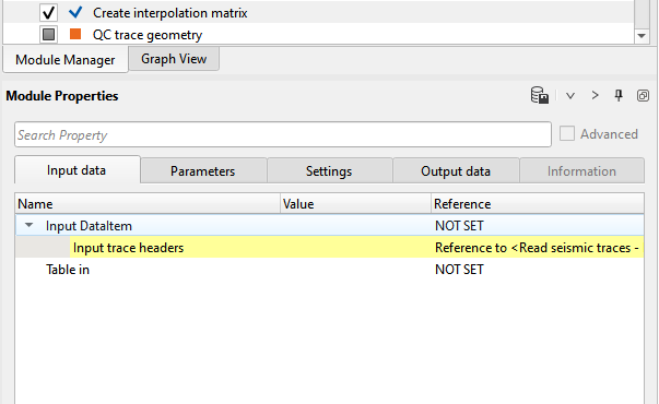
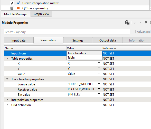
3) Create interpolation matrix This module is used to provide the water depth information to predict the multiples. In the Multiple type parameters, we have two options as we explained in the parameters section above.  

If the choice of Multiple type is Water depth then Select Water depth option and connect the Bottom depth matrix to Create interpolation matrix. This module is very useful in creating any matrix index. We've two options to get the information from.

1. Trace headers

2. Table

If the input should be taken from the trace headers the user should reference/connect to Input trace headers. Otherwise, choose the Table in and select the appropriate table if there is any.

4) QC trace geometry This module is optional module. Prior to proceeding further, it is always better to QC the data. QC the input data for SOURCE_DEPTH, RECEIVER_DEPTH, SOURCE_WDEPTH and RECEIVER_WDEPTH information to see whether they are existing or not. This module is not limited to these trace headers. This can be used extensively to QC all the trace headers information to make sure that the right trace headers information is passing to the next phase of processing.

5) Read seismic traces reads the input file name with both primaries and multiples i.e. 0020-denoise-gathers. Execute the module by double click on it or press on run button from the upper menu.

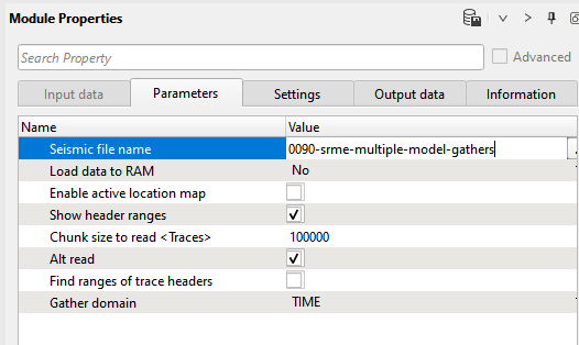
6) Read seismic traces This module is to read the predicted multiple model. Choose the gather 0090-srme-multiple-model-gathers

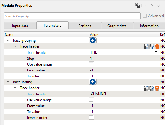
7) Sort traces Here we need to sort seismic traces for Seismic loop. Add Sort traces module and set FFID header for Trace Grouping and CHANNEL as Trace Sorting as it is shown below

8) Seismic loop Connect trace headers vector (Input sorted headers) from the Sort traces module output and seismic (Input SEG-Y data handle) from Read seismic traces.

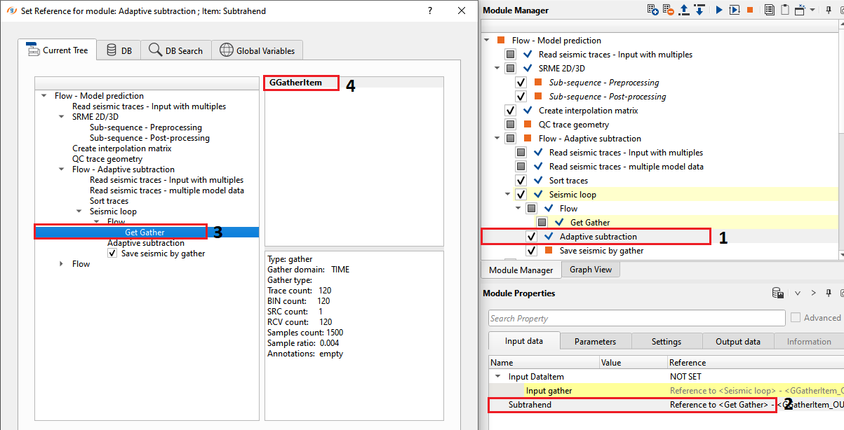
9) Adaptive subtraction This is the second stage of SRME where we adaptively subtract the multiples from the input data using predicted model. Adaptive subtraction module requires two inputs. One is the actual data which got both primaries and multiples. The second one is multiples predicted model. For the same, we've read both inputs (input data and multiple predicted model) using Read seismic traces module. Since the adaptive subtraction is inside the Seismic loop module, the first input is automatically connected by itself. The second input we need to add to manually as shown below.

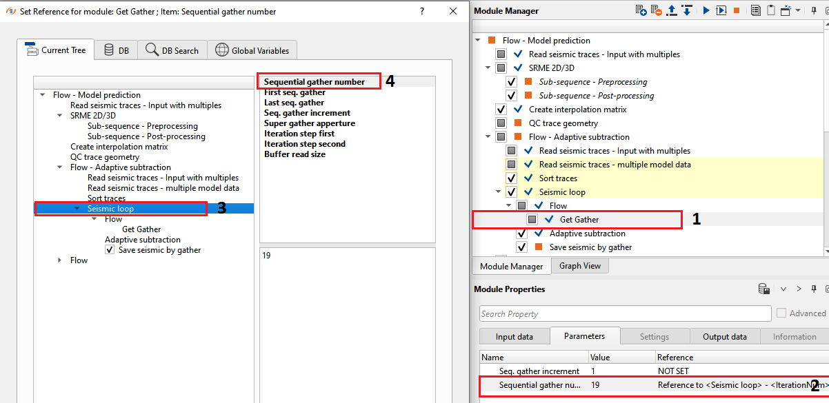
To reference/connect the second input, we should add a module Get Gather inside the Seismic loop.

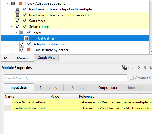
We make the connection/reference of GReadWriteGFilItem to Read seismic traces - multiple model data. Similarly, we make the connection/reference to GGatherIndexVectoritem to Sort traces module. In the parameters of Get Gather, we need to make the reference to Seismic Loop as shown below.

Now we connect this Get Gather output gather as a second input to Adaptive subtraction module.

10) Save seismic by gather is used to save the seismic data in g-Platform’s internal format with .gsd extension. This module should be used within the Seismic Loop. Write a name of output seismic data set 0090-srme-output-gathers and Seismic loop on the entire data set by using launch all modules button.  Make sure to  Turn off all difference calculations prior to launch  srme workflow for the entire seismic data.