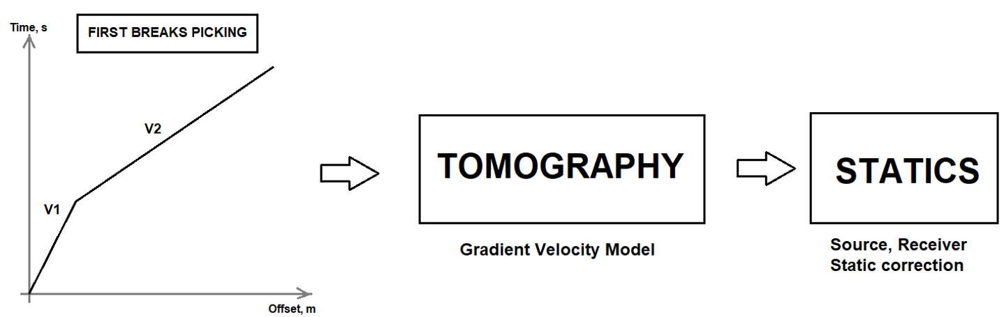
Statics calculation that based on the refractions methods requires first breaks as mandatory input data set. Therefore, we need to do a picking of the first arrivals (guide-wave) on the input seismic traces. For this task g-Platform has Refraction FB picking - azimuthal solver guide / phase / aperture module, then we need to calculate statics corrections by using this regression method solving or use tomography algorithm Tomo statics 3D.

A brief common sequence description of statics in g-Platform system:

STATICS solution (both refraction and residual) is a two steps process in g-Platform that consists of:

•        Calculation

•        Application

STATICS CALCULATION:

For refraction statics calculation we have two different solutions (modules) available in g-Platform.

1.        Refraction FB Picking – Azimuthal Solver guide/phase/aperture

•        In this module, we calculate low, high and middle frequencies or in other words – the short and the long wavelength statics.

•        This module has extensive manual and automatic first-break picking capabilities

•        To calculate these statics, we need to pick the first breaks.

•        There is an option to calculate the residual statics (activated by check box Find residual)

•        This module is essentially a 3D, while 2D handled as a private case

•        This module has an azimuthal term that allows to have more complex (azimuth-variant) solution.

2.        Tomo statics 2D or 3D

•        This algorithm works on Fresnel seismic travel time tomography.

•        The input is first-break picks to compute the statics solution.

•        A Fresnel volume is defined as a set of many waves delayed after shortest travel time by less than half a period. Thus calculating the travel times from both source and receiver. By using finite difference method we solve the eikonal equation.

•        There are 2D and 3D variations of this module for corresponding seismic data type

3.        Refraction statics - cross correlation – innovative proprietary approach

•        This algorithm based on cross-correlation between near offset traces

•        The cross-correlation made along refraction wave travel-time, amplitude and waveform

•        The high frequency statics resolved as part of the solution

•        Implemented for 2D and 3D planned during Q3/2022

STATICS APPLICATION:

•        The application of statics to the gathers made by either of two modules depending on which refraction (or residual) statics was deployed:

➢        Apply statics shifts – designed for statics item (library) without azimuthal term (such as output from Tomo or Cross-correlation statics or Residual statics)

➢        Apply azimuthal statics shifts – designed for statics item (library) with azimuthal term (such as output from Refraction FB picking)

➢        Weathering/drift statics – designed to make a layer replacement based on Velocity from refraction statics modules. Implemented for more standard approach of working with Tomo statics.

•        Once the statics are calculated from any one of the methods above, we apply these statics:

➢        Before or after NMO, for VA or within other applications. That can be done with or without saving the gathers to a disk

➢        Saving to a disk: this is more standard way of doing it and as such require a data set (even if temporary) to be saved to a disk for any test of statics

➢        Without saving gathers to a disk: this is unique feature of g-Platform that allows to apply statics (and other processing) on fly without storing the data to a disk. As a result, it takes a bit more calculation time to see the result, but optimize substantially storage/disk use and time for a testing.

•        As mentioned just above, to evaluate the statics response we apply them within the Stack Imaging module to QC the stacks without need to create a separate set of gathers – that provides a huge optimization in the project progress.

•        In Stack imaging, there are several points for applying statics (or any other modules that have gather-in and gather-out):

➢        For VA : the statics applied selected CDP gather before calculating velocity semblance. That will not change the result, but only the vertical velocity panel where we are making the picking

➢        Before NMO: the statics applied to CDP gathers when running Stack imaging before NMO was applied. That is very convenient method of testing statics, since does not require saving to a disk

➢        After NMO: the statics applied to CDP gathers when running Stack imaging before NMO was applied. That is very convenient method of testing statics, since does not require saving to a disk

➢        To clarify: [Stack imaging] doesn’t calculate any statics, it only facilitates to apply any processing sequence. This module is used to pick the velocities, picking mutes and creating stacks. Once we create the stack, we can shift the data to final datum using shift datum parameter within the Parameters of Stack Imaging module.

•        Similarly the statics can be applied in other sub-sequences of different applications, such as PSTM, PSDM, SC amplitude correction, SC Deconvolution, etc…

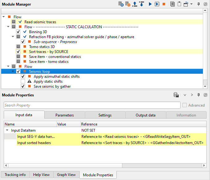
•        When applying statics to the gathers that will be stored to a disk, we usually would use one of following applications/flows: Seismic loop, Distributed seismic loop, Loop and sub-sequent use of Save seismic by gather or Save seismic modules.

Refraction FB picking - azimuthal solver guide / phase / aperture

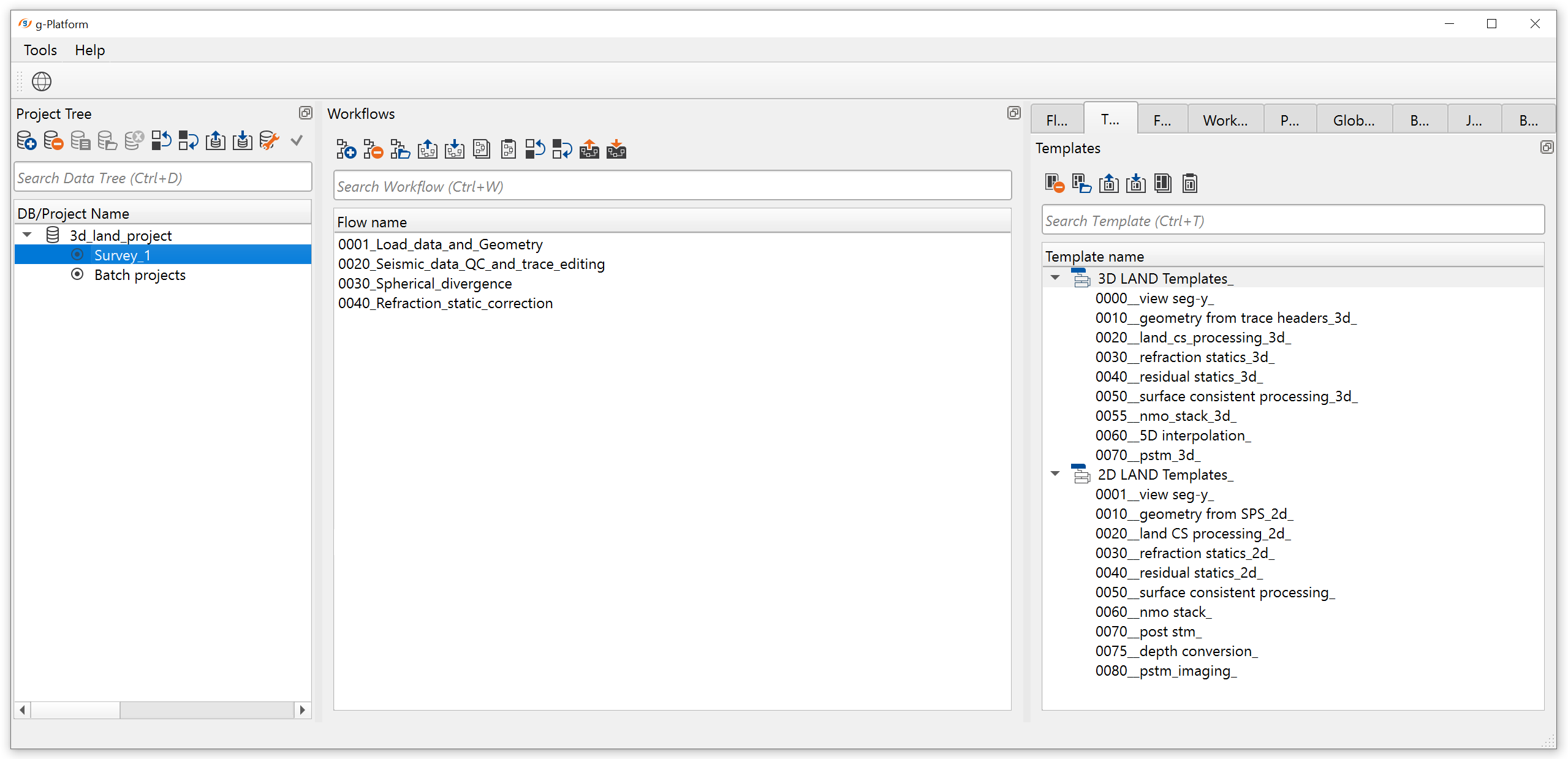
Create a new workflow 0040_Refraction_static_correction:

Notice, that tomography procedure requires high quality picks, so it is better to have accurate manual picking on the line (manual picking if you have enough time). The seismic is vibro data and it is another obstacle of using auto picking method as well as trying to use tomography procedure, the result may be far from being sufficiently addressed in comparison with the conventional reciprocal method static solution.

Let’s fill-up the workflow with all necessary modules for static calculations:

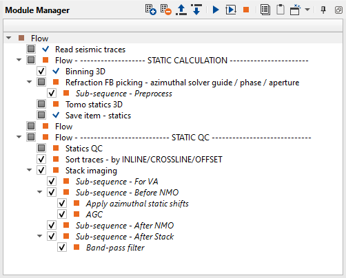
1. Read seismic traces - loading seismic data for picking

2. Binning 3D - we will use topography map from this module

3. Refraction FB picking – azimuthal solver guide / phase / aperture – manual or auto picking of the first breaks

4. Tomo statics 3D – tomography statics calculations

5. Static QC – quality control for statics from Tomo statics 2D/3D

6. Sort traces - sort traces by INLINE/CROSSLINE/OFFSET for stacking

7. Stack imaging - create a stack, make QC of refraction statics

1) Read seismic traces. For the first break picking step we should use seismic without any processing in order to have original first response from guide-waves. Load seismic data set 0001_Geometry.

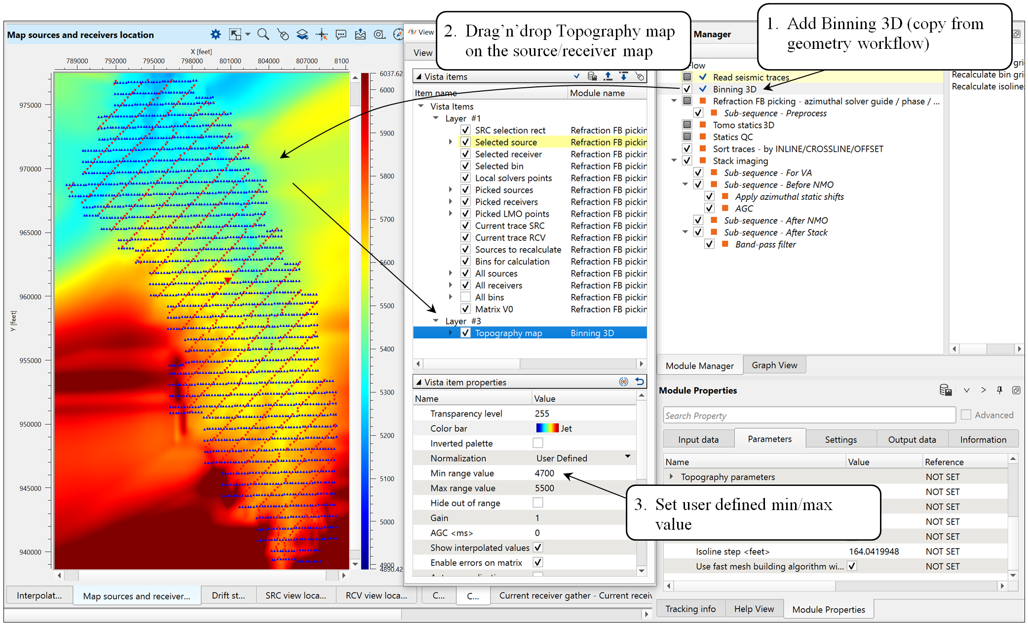
2) Binning 3D. Just make a copy (ctrl+c -> ctrl+v) of this module from the geometry workflow (0001_Load_data_and_Geometry). We will use original topography map from this module for LMO picking QC.

3) Refraction FB picking - azimuthal solver guide / phase / aperture. This module computes the static correction based on the first breaks of the data. It allows the user to interactively pick or correct the automatically picked first breaks. Subsequently, the first breaks can be used to solve for a refraction static solution generating a static correction for the source and receiver positions. The module calculates only the refraction correction, that is, replacing the near surface low velocity layers from the surface to the base of the calculated near surface. The module does not include an elevation correction, a shift to correct the data from topography to final datum. This correction to final datum is performed with a separate module Shift Data. Since most processes in g-Platform that would require the statics applied (for example NMO) can be run from topography, being able to easily separate the refraction correction from the final datum correction is very useful. How to use floating and constant datum planes will be discussed in the end of this chapter.

Refraction FB picking uses the picked first breaks and user provided parameters for the solver to calculate the source and receiver static correction at each surface location. The solver includes options to calculate a smoothed solution, as well as to solve into multiple azimuths. Additionally, a residual correction can be calculated and applied at each source and receiver giving a short-wave correction. The replacement velocity is calculated internally by the module. Upcoming changes will allow for the user to specify a weathering velocity as well as a replacement velocity. With these parameters specified the module will build a near surface weathering model and then use the user defined values to compute static corrections.

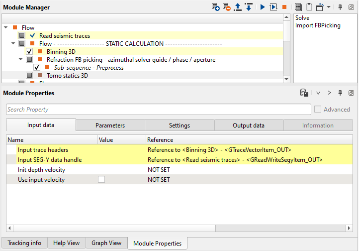
Fill the Refraction FB picking – azimuthal solver guide / phase / aperture parameters before performing calculation and displaying the data set. For the training seismic we will use the following example, but you should do some extra tests by changing parameters for better understanding:

Input data:

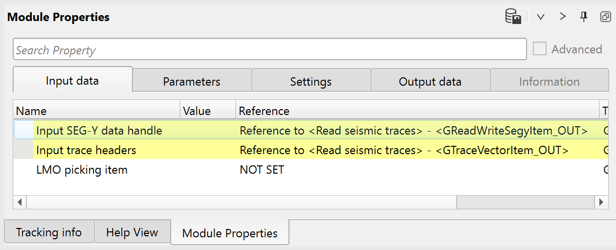
Parameters:

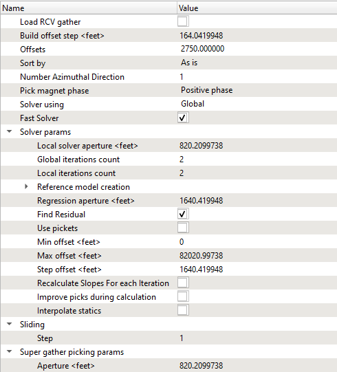
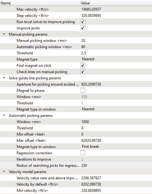
Let’s have a look at the main parameters we need for picking:

Load RCV gather

By default, it is FALSE. If checked, it will display the receiver gathers in the current receiver gather window.

Build offset step

Provide the offset step size. Depending on the offset step size, it will build the offset classes that can be chosen from the Offsets option parameter.

Offsets

Select the desired offset from the available drop down menu.

Number Azimuthal Direction

By default 1. In case of 3D, the user can define the azimuths.

Pick magnet phase

Provide the phase to pick the first breaks.

Min offset

Provide the minimum offset value for picking the first breaks.

Max offset

The user can limit the minimum and/or maximum offset values. Provide the maximum offset value for picking the first breaks.

Step offset

Offset step size. Create an offset class as a group of offsets for velocity estimation.

Sliding step

Provide the sliding value to jump to next source/receiver gather.

Super gather picking params:

Improve picks  – Set picks more accurate on phase if it possible.

Aperture

Super Gather Aperture, the aperture of locations that will be picked on either side of the current pick.

Min velocity

Minimum velocity range for super gather picking.

Max velocity

Maximum velocity range for super gather picking.

Step velocity

Step velocity between minimum and maximum to be used for super gather picking.

Run local solver to improve picking

Leave checked to use the results of the local refraction statics solver to improve the results of your super gather picking.

Improve picks

Set picks to be more accurate on the phase if possible.

Manual picking params:

Manual picking window

Search window used for manual first break picks.

Automatic picking window

Search window used for in automatic super gather picking mode.

Threshold

Threshold for manual picking.

Magnet type

Phase of first breaks to be picked.

Find magnet on click

Type of energy for first breaks.

Check lines on manual picking

By default TRUE.

Solve guide line picking params:

Aperture for picking around existed picks

Provide the aperture value for picking first breaks using the solve guide line with existing picks.

Magnet to phase

Choose the phase for picking the first breaks. By default, FALSE. If checked, the next two parameters Window and Threshold will be activated.

Window

Provide the picking window.

Threshold

Define the threshold. By default 3.

Magnet type in window

By default, Nearest.

Automatic picking params

Window

Search window for automatic first break picking.

Threshold

Provide the picking threshold value for automatic picking.

Min offset

Provide the minimum offset value for first break picking.

Max offset

Provide the maximum offset value for first break picking.

Magnet type in window

There are multiple magnet types are available for first breaking picking. By default, Nearest.

Regression correction

By default, FALSE. If checked, next two parameters will be activated.

Iterations to improve

Provide the number of iterations to improve the regression correction.

Radius of searching picks for regression

Provide the search radius.

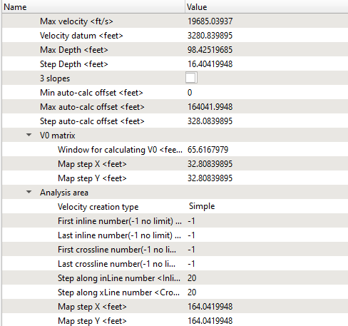
LMO params

LMO type

Type of LMO to be applied to shot and receiver gathers for picking:

None - indicates no LMO will be applied;

V const - is a constant velocity LMO as indicated by the V LMO parameter;

Picking - will apply an LMO based on the bin gather picks.

Further step is setting up your work area, it means to make an configuration of all necessary Vista Windows for QC and interactive engagement. Click RMB on the module -> Vista Groups -> All groups > In new window:

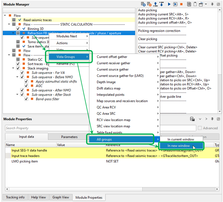
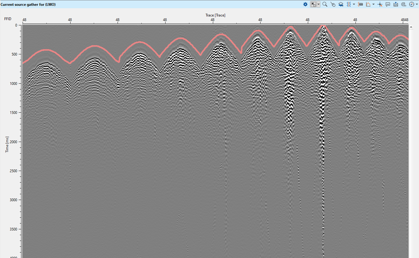
The first Vista Window we are going to use is a Linear Move Out (LMO) correction on the Source gather view. The LMO one of the main parameters for FB picking in the view of the fact that it is used as a guide function for auto picking. Consequently, we should pick LMO guide function on a few source gathers on different locations. Picking may be exactly on the first arrivals or a little bit above them, it depends on what option (algorithm) and parameters you use for auto picking.

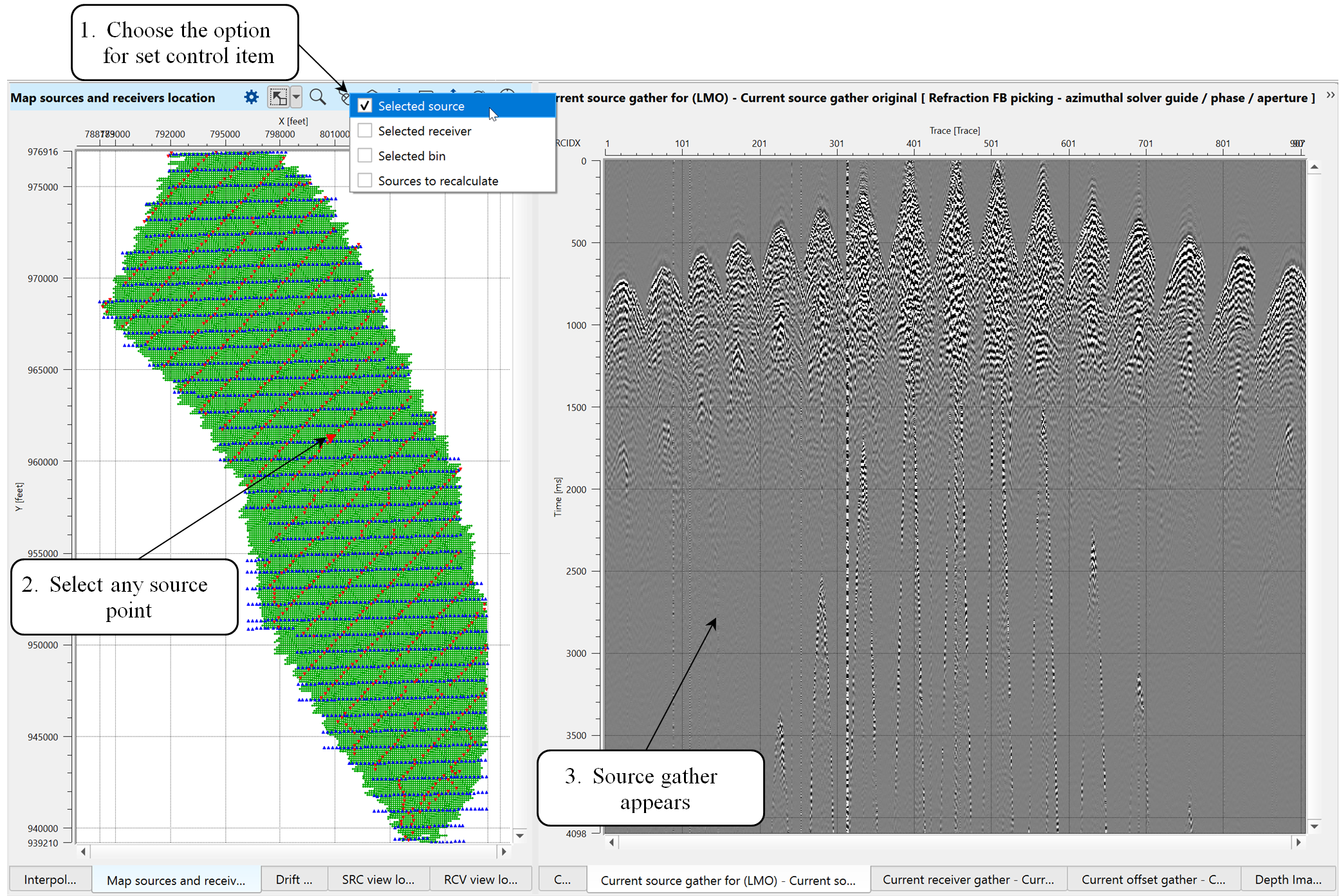
After connections of the input data, we can see a map of source and receivers. This map is interactive, it ans you can click on any source/receiver/bin and it will be appeared on the gathers view:

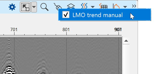
Activate LMO trend manual set item control and pick LMO function for several source points through the the entire survey, pay attention on a big elevation differences, because at those location you should correct LMO trend function:

Pick LMO function:

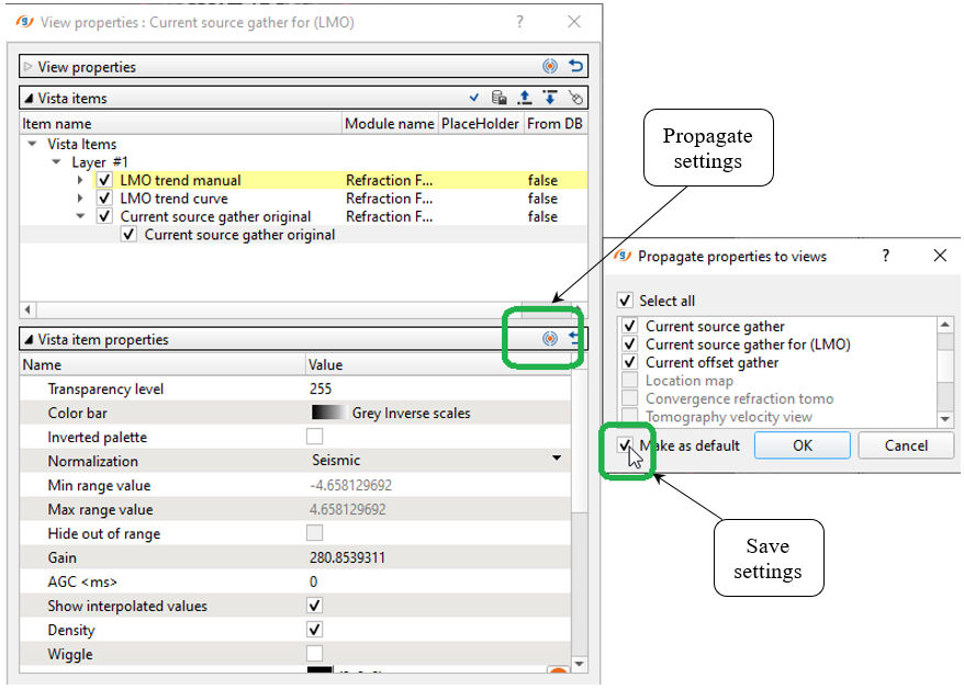
All the visual setting were configured and we can propagate and save them:  

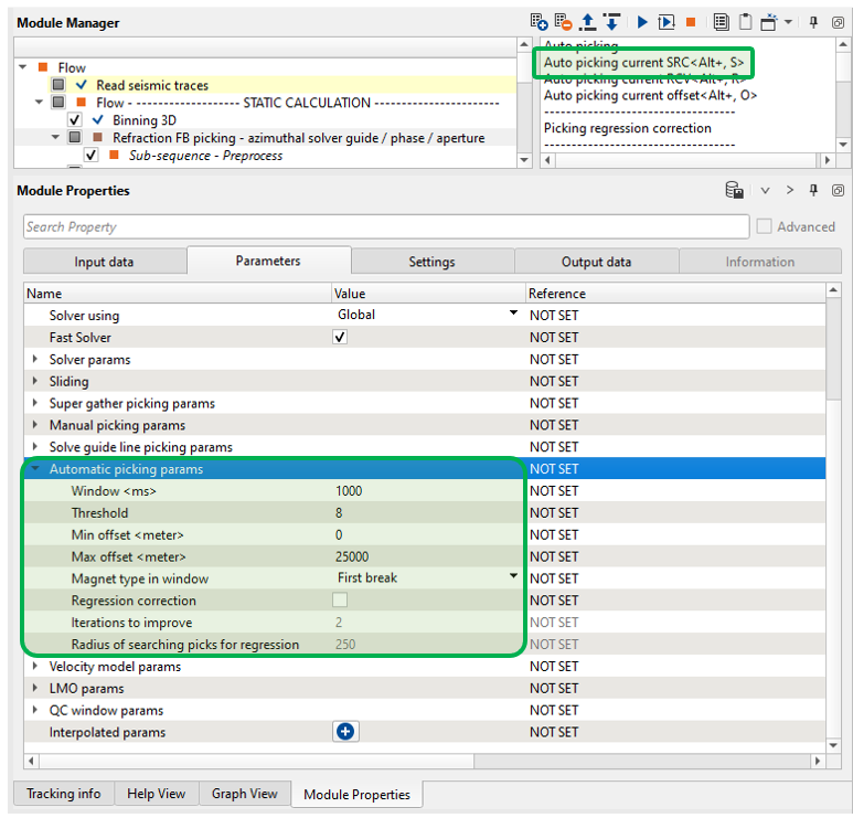
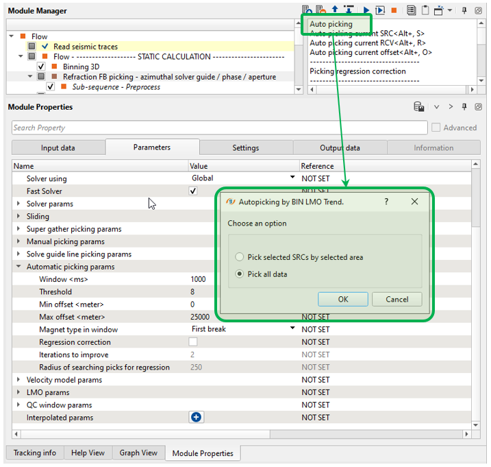
Next, open the source gather FB picking window and execute one source FB picking by pressing Auto picking current SRC<Alt+,S> button (in the Action menu):

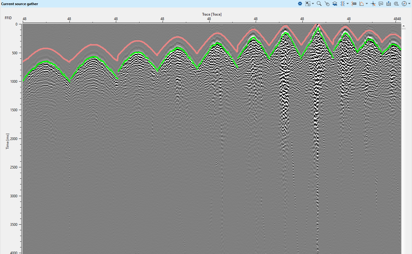
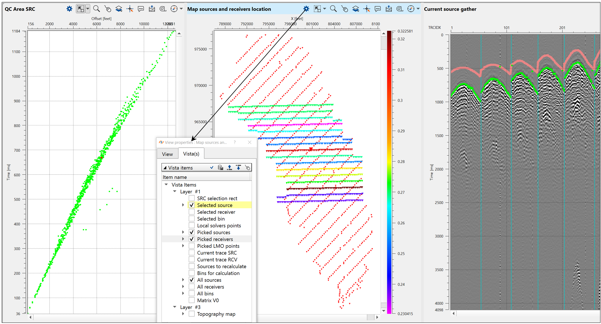
In the above image, we can see that the green dots are the automatic picking by using the automatic picking parameters. In case we wants to make any changes to picks, select the manual picking option SRC manual control from the control item and do the manual picking to adjust the badly picked picks. Please adjust the manual picking parameters as per your input data. Also we see blue vertical lines. These lines are receiver line separators.

Then we are going to run auto picking for the entire data set by clicking on Auto picking action button:

Eventually we have all FB picks and need to check it, open the Map sources and receiver location and activate Selected source option:

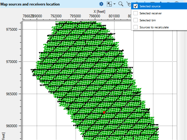
Pay attention of the aperture area QC that we can increase or decrease by using its parameter:

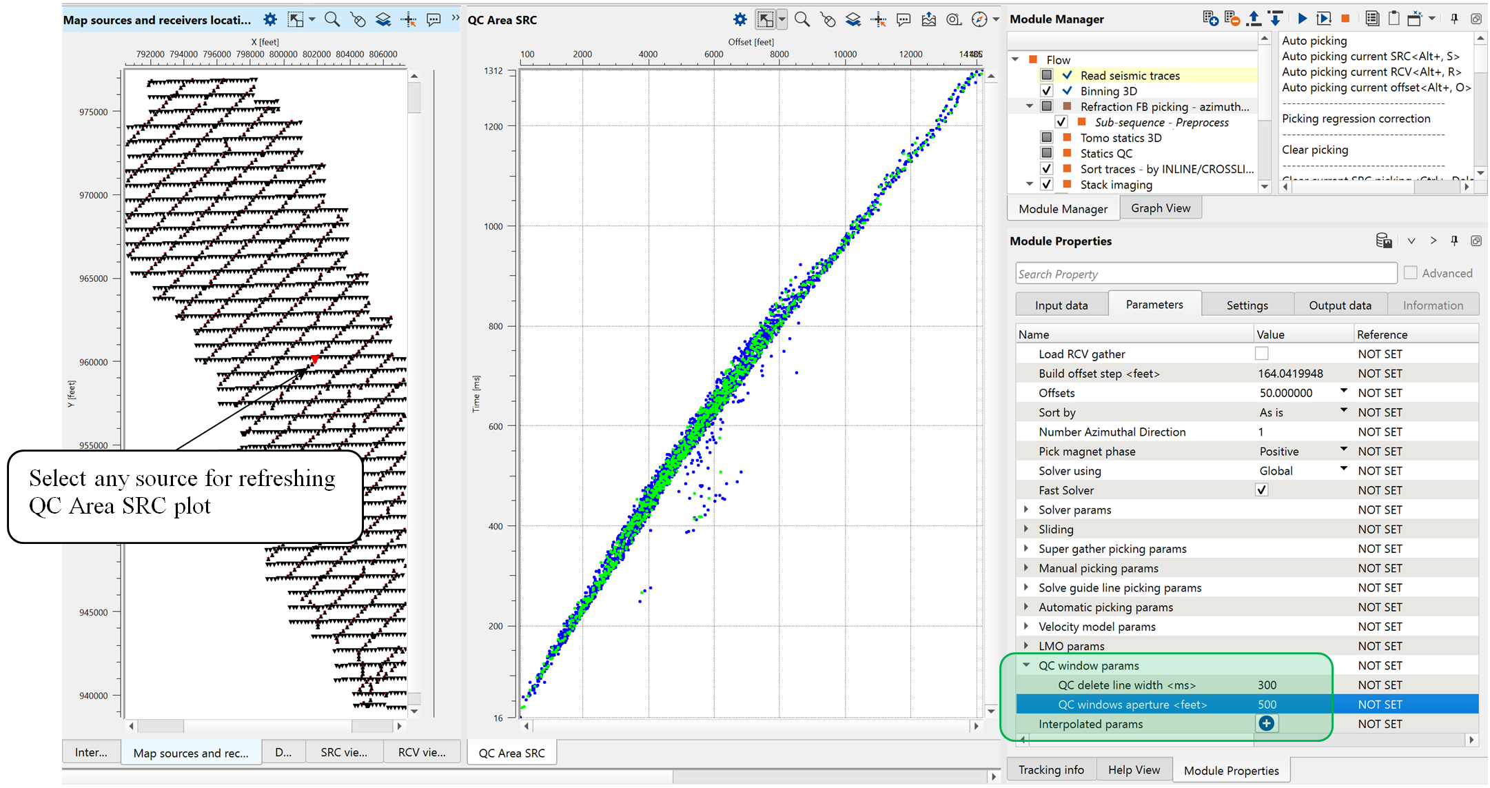
Change QC aperture back to 1000000 and let's figure out what we have:

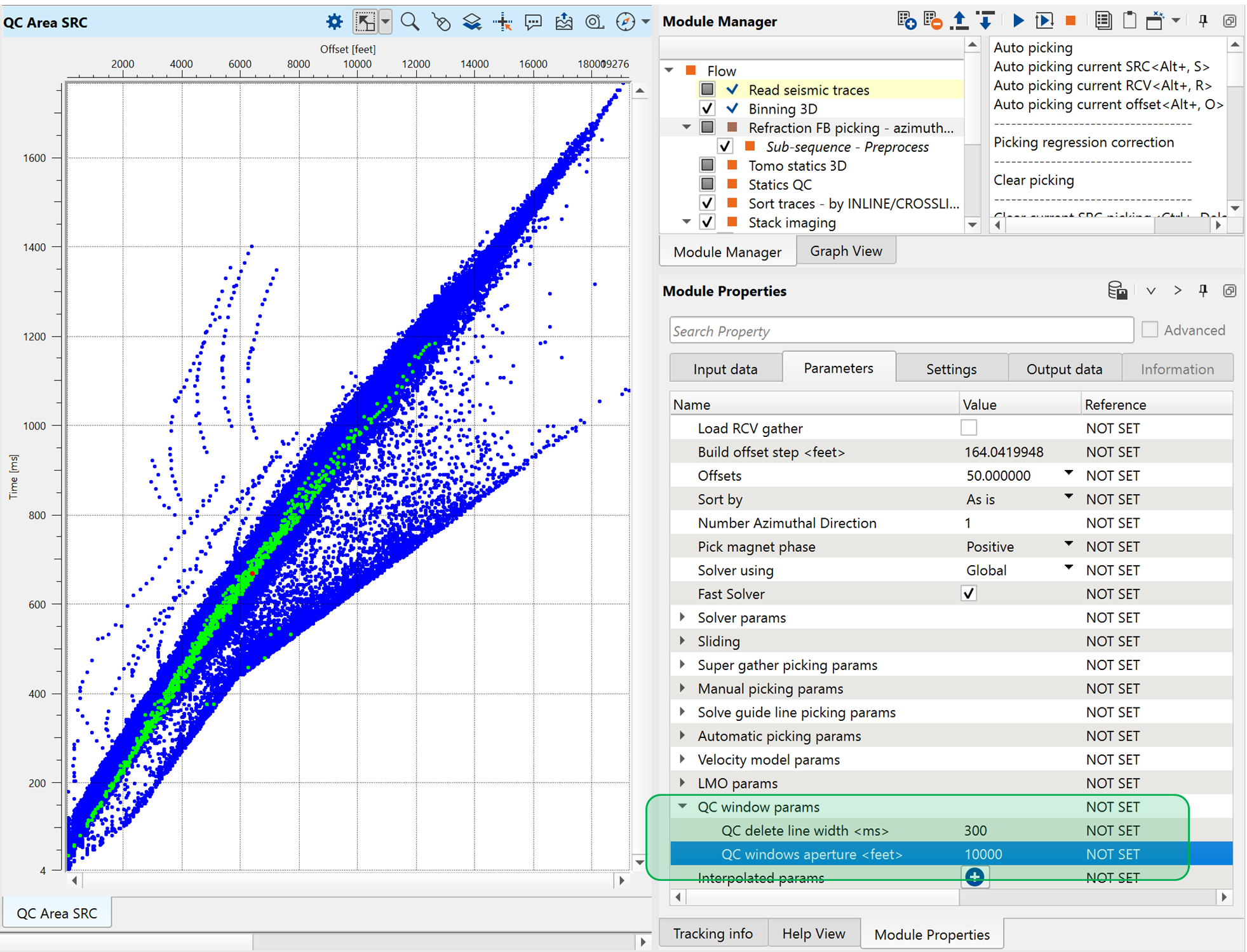
Remove 3-4 sources picks and select some outline pick to see what we have next (also we will delete those sources on the next steps, so write down source numbers):

So, there are some few bad picks on the gather. We have several options to resolve the problem of bad picks: 1) test auto pick parameters and re-run the auto picking, 2) correct bad picks manually, 3) remove bad pick via QC Area SRC window. In this case, we are going to use the last method: remove bad pick via QC Area SRC.

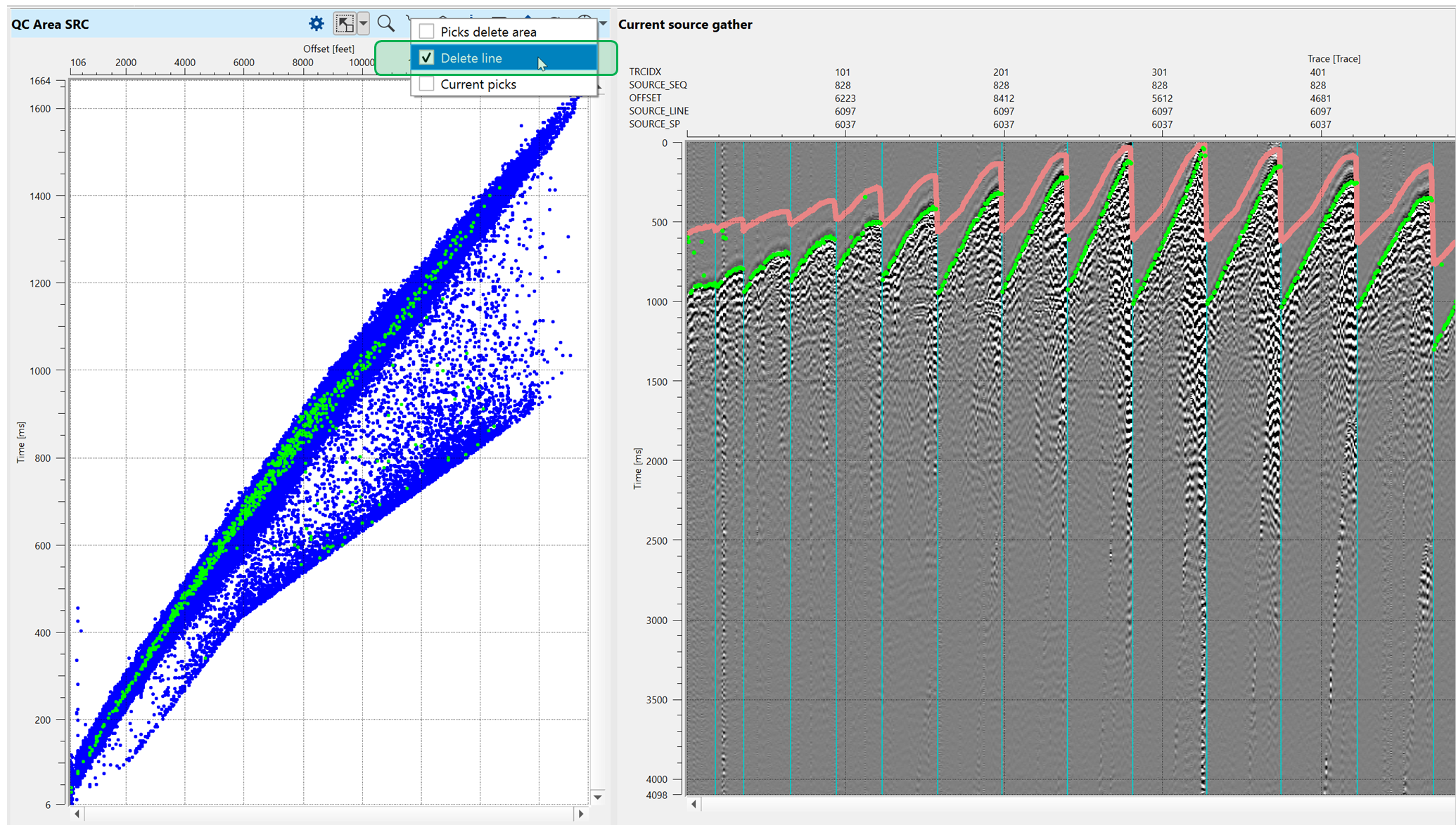
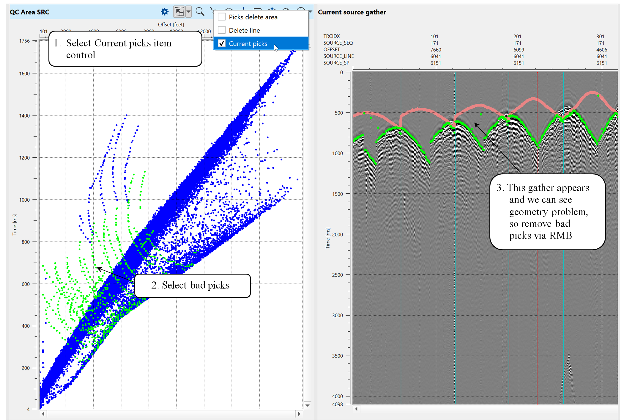
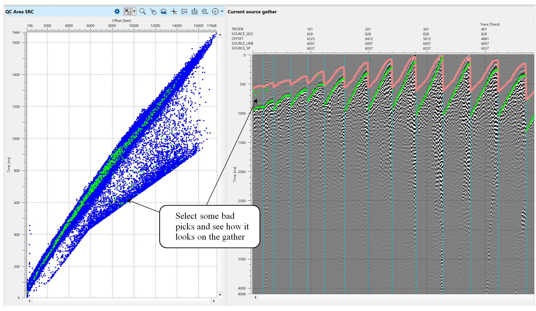
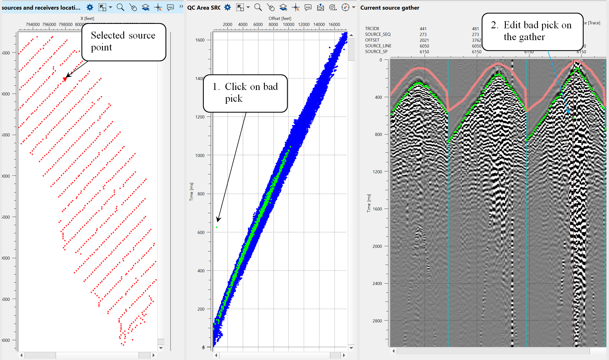
Now we can choose any source from the location map and perform FB picks QC and editing. Other windows are connected to each other automatically, so it allows to perform interactive QC on fly.

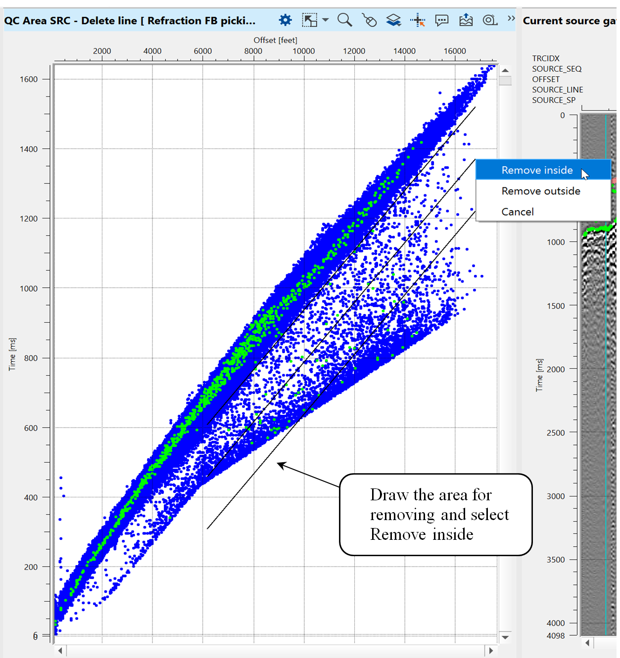
Once we selected the Delete line option from either QC Area SRC or QC Area RCV the next step is to remove the outliers or the bad first break picks. Use hold and drag MB3 or RMB to get 3 parallel lines as shown below. Once we decided the area that must be be deleted, release the MB3 or RMB. Upon releasing the mouse, it will come up with 3 options (Remove inside, Remove outside, Cancel) as shown in the below image. Since we want to delete the set of outliers and it is inside the 3 parallel lines, we need to choose Remove inside. With that selected option, it will remove/delete all the picks inside the 3 parallel lines as shown below.

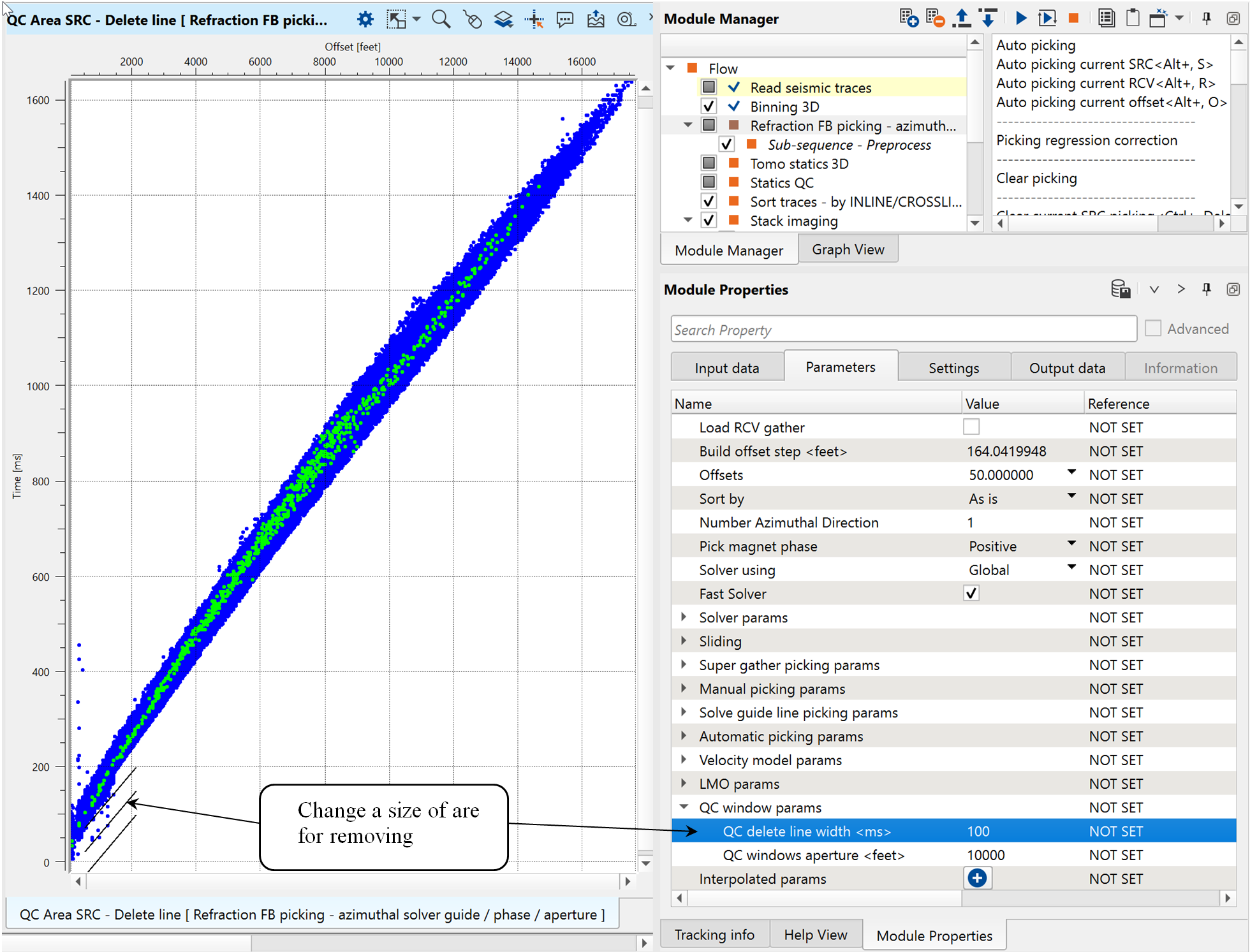
Use size parameter for increase/decrease the area:

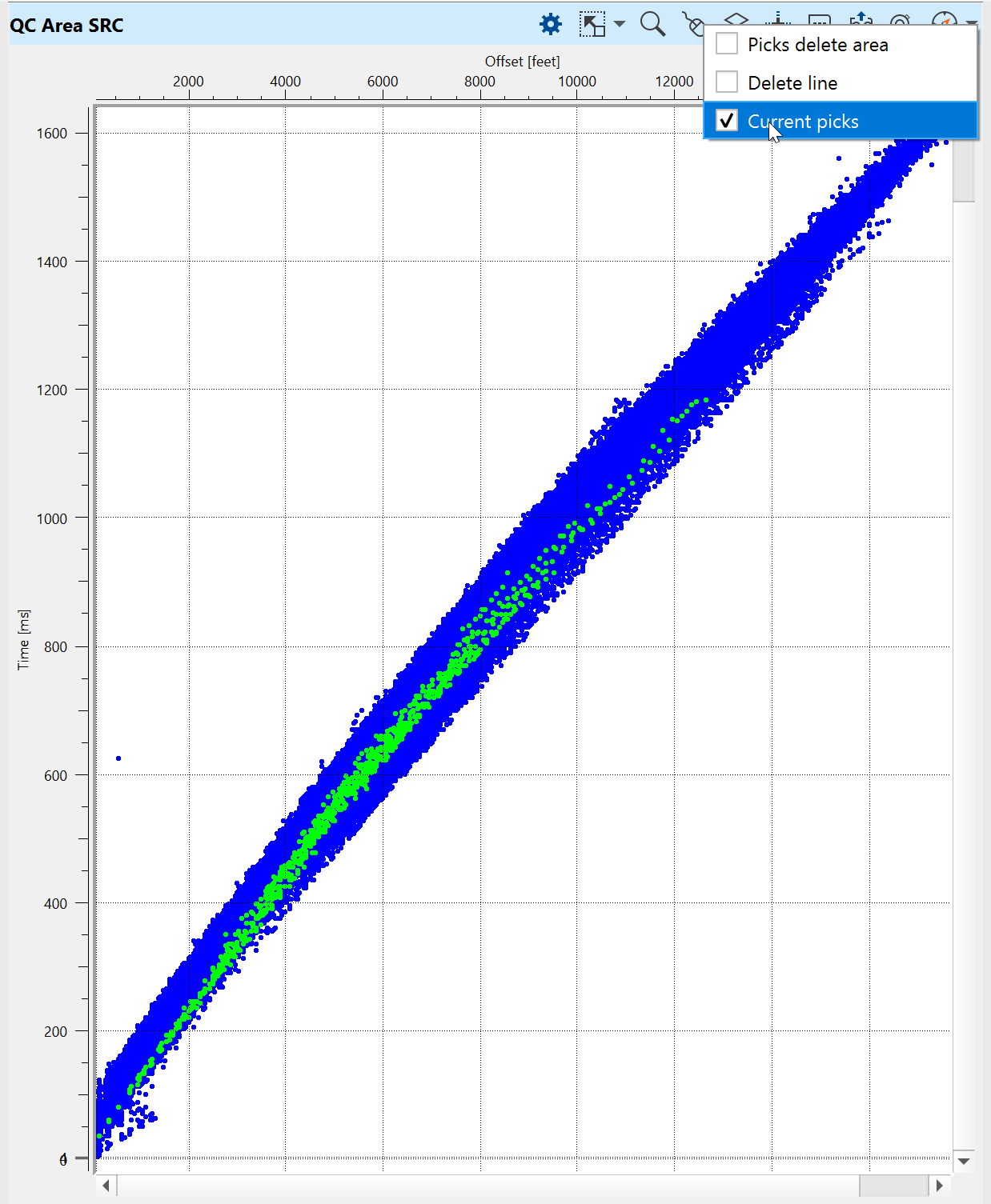
Or choose another option for picks removing Current picks (as shown below). Once we select this option, it will automatically select particular pick on the Current source gather and marks the pick with a red vertical line. Now we can manually edit this bad pick:

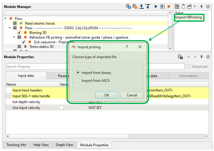
The final step is export FB picking to binary file that we will use for tomography process. Find Export picking action and choose Save in Binary, because tomo statics module requires binary format:

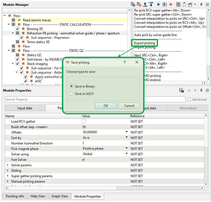
Define a name of the output binary file FBpick, we will use this file in the next step - tomography.

Now we have all FB picks and there two options for static calculation, by using:

• Refraction FB picking – azimuthal solver guide / phase / aperture;

•Tomo statics 2D/3D.

Execute Refraction FB picking – azimuthal solver guide / phase / aperture, now we have refraction static correction and it is easy to do a QC. Go to vista window Current source gather and do a quick statics QC:

It was a fast QC of static corrections calculated by Refraction FB picking – azimuthal solver guide / phase / aperture. Of course we are going to calculate stacks, but before we do it there is another option for static calculation by using tomography - module Tomo statics 3D. By the way, static corrections located in current workflow (in the module), and we will save it later.

Tomo statics 3D

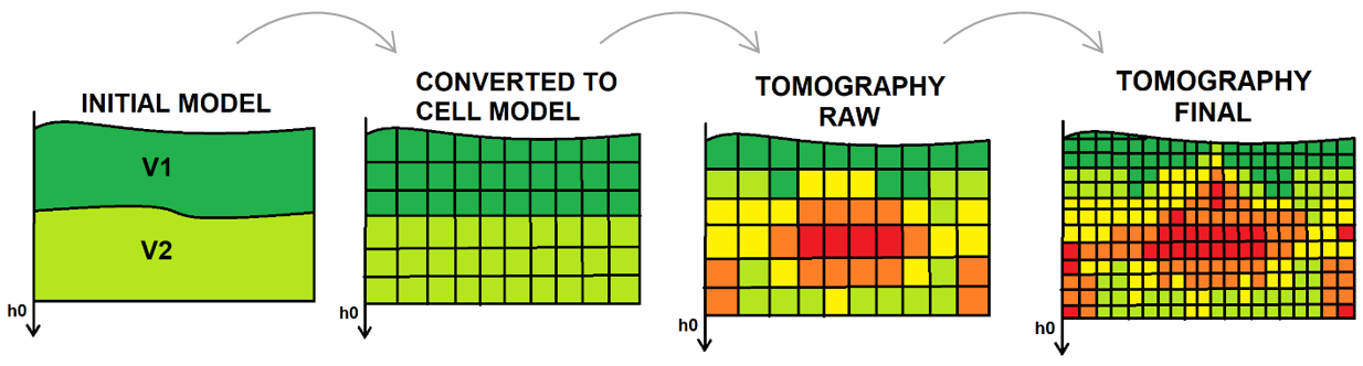
4) Tomo statics 3D. Tomography plays a key role in seismic imaging. Be it is a building depth velocity model or calculating the refraction statics by generating the near surface model. Refraction Tomography statics are used in the event of regular refraction statics are not giving optimum results or to improve the refraction statics solution. In this method, the weathering zone (WZ) is parametrized as a number of cells that used for filling up a depth velocity model. Travel times are goes through the cell-model, and residuals times are converted into velocity variations in 2D/3D cells. Here we are able to calculate vertical velocity gradient due to the fact that tomography is a nonlinear move out modeling of the first arrivals. 

The tomographic is sensitive to the initial model due to the fact that the nonlinear solution performs by iterating the ray trace calculation and velocity is updated by local linearization, so the solution of tomography is depending on quality of first breaks picking. 

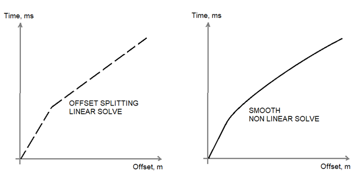
Linear (left) and nonlinear (right) solutions comparison:

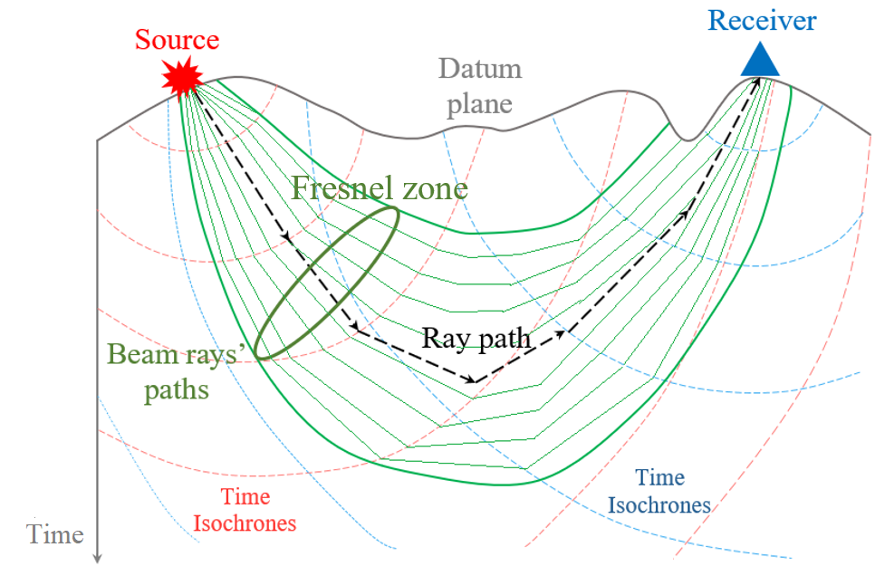
The tomo-statics modules in the g-Platform system are based on the Fresnel seismic travel time tomography. A Fresnel volume approach is applied to represent wave propagation for seismic travel time tomography instead of rays. A Fresnel volume is defined as a set of many waves delayed after the shortest travel time by less than half a period. It is derived by calculating travel times both from a source and from a receiver. Tracing rays from sources to receivers is completely avoided.This considerably reduces computational time. We solved the eikonal equation by using a finite-difference method to calculate travel times. The advantage of this approach is as follows: first, the frequency of wave can be introduced into analysis. Therefore, we can evaluate the resolution of seismic tomography. Next, the smoothing feature can be naturally introduced. Finally, Fresnel volumes with finite bandwidth considerably reduces the sparseness of ray distribution.

The more physically-realistic representation of wave propagation is to treat a ray path as a beam with finite width. Using a Fresnel volume is a natural and an effective approach. A Fresnel volume is a set of many rays delayed after the shortest travel time by less than half the period of wave. The rays in a Fresnel volume are added constructively to form the first-arrival of wave. There have been several studies on the application of Fresnel volumes to seismic tomography since Harlan (1990). In this study, first, we discussed the characteristics of Fresnel volumes. Next, we formulated the inversion procedure. Then, we investigated the resolution of tomography with respect to the frequency (Toshiki W. Seismic travel time tomography using Fresnel volume approach).

Travel times scheme:

A module Tomo statics 3D is used for tomography and it requires the first break picks. In this module, it starts with an initial model and performs updating the model during each iteration until it converges to the best solution.

Scheme of tomography steps:

Demo data also consists of the FB picking file on your disk in the same folder with the input seismic data set, but you just need to convert ASCII FB pick file into Binary one via Refraction FB picking - azimuthal solver guide / phase / aperture module (import->export). So, we can use the module Tomo statics 3D which requires first breaks as mandatory input data set.

Tomography procedure requires high quality picks, consequently preferable to have manual picking on the 3D line due to relatively small amount of source gathers. The seismic is vibro data and it is another obstacle of using auto picking method as well as trying to use tomography procedure, the result may be far from being sufficiently addressed in comparison with the conventional reciprocal method static solution.

We will use Tomo statics 3D module For tomography procedure , add it to the workflow RMB->Modules Next->Find module->Tomo statics 3D and set all the parameters.

Input data:

Connect all the input data vectors from the previous module and import the FB pick binary file:

Tomo statics 3D module calculates necessary grid automatically in accordance with the input trace headers, buy can use any grid if necessary (use optional parameters: Use provided bingrid + Output geometry).

Usually, testing parameters starts with wide cells size of the model, because initially the main goal is to find the most appropriate values for other parameters. When we have optimal result, it is reasonable to reduce cell size and increase the number of iterations. Eventually, a dense/high resolution gradient depth velocity model is calculated as well as static corrections (ms) for sources and receivers. A depth velocity model may be used for the depth migration step as the upper part of the PSDM model.

Parameters:

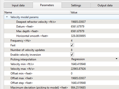
Tomography parameter explanation:

Velocity model params:

Definition cell-velocity model.

Deepest refractor velocity - the maximum values of guide-wave.

Datum – start value for tomography calculation, constant datum.

Max depth – maximum depth in meters of the model.

Horizontal smooth – horizontal velocity smoothing in meters.

Frequency:

Parameter for making solution more detailed in terms of travel time decomposition, bigger value – more detailed result (high spatial frequency), but time consuming. Pay attention on figure 3 Travel times scheme, green constrain depend on this parameter, less frequency - smoothie result.

Number of velocity updates

Tomography iterations.

Enable velocity inversion

Allows to have velocity inversion on the model.

Picking interpolation:

Options for interpolation missing first breaks picks:

Nearest – get picks from the nearest traces, use it in case of small gaps in FB picks.

Regression – model picks by using regression method.

Velocity min

Value for making minimum velocity constrain (m/s).

Velocity max

Value for making maximum velocity constrain (m/s).

Offset min

Value for making minimum offset constrain (m).

Offset max

Value for making maximum offset constrain (m).

Offset step

Step for splitting offset by classes (m).

Maximum deviation (picking to model)

Maximum variations of observed picks according into the model trend.

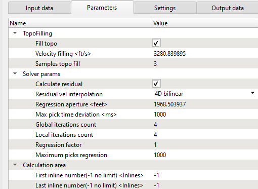
TopoFilling:

Visual parameters for displaying velocity model, it is not used for calculations:

Fill topo

Values above the relief elevations for filling.

Velocity filling – define exact value for filling.

Samples topo fill – how many samples to fill.

Solver params

Residual statics solver parameters:

Calculate Residual - By default checked. This will allows to calculate the residuals.

Regsidual vel interpolation - Choose the velocity interpolation method. By default Spatial regression however we recommend using 4D bilinear.

Regression aperture - Value of aperture for regression algorithm (m), bigger value – smoother solution.

Max pick time deviation - Maximum picking variations (ms) for residual static solution.

Global iteration count - Number of global iterations for residual static solution.

Local iteration count - Number of local iterations for residual static solution

Maximum picks regression - By default 1000. This parameter is obsolete.

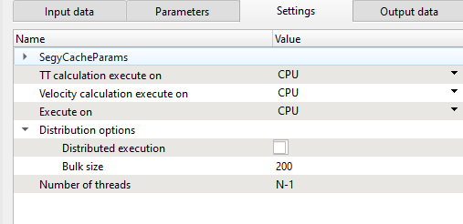
Now we have defined all the parametrization and the next step is launching the tomography calculation by double LMB click on the module. Use CPU and distribution mode for time consuming procedures or big acquisition. Those functions must be configures on a cluster by your system administrator. Tomo statics 3D is a CPU only (cluster based) and doesn't work on GPU at the moment.

To visualize the tomography velocity model and convergence, we should open the vista items. The module generates many QC windows: Current source/receiver gather, Tomography velocity view inline, Tomography velocity view crossline, Convergence refraction tomo and Calculation area.

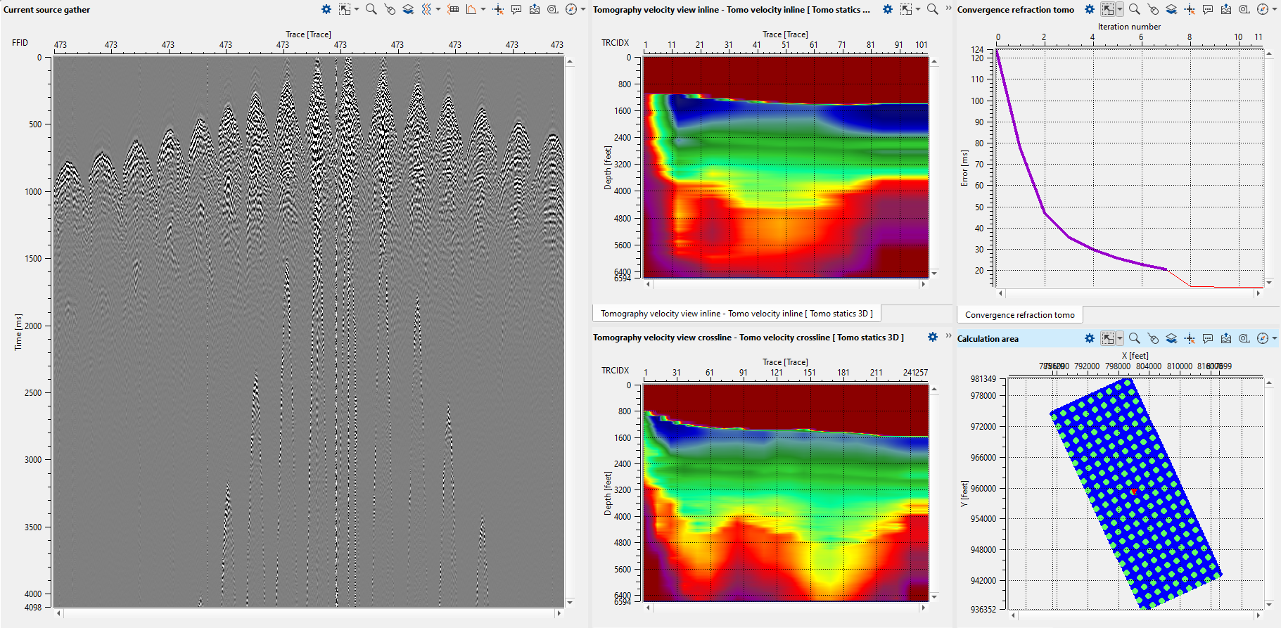
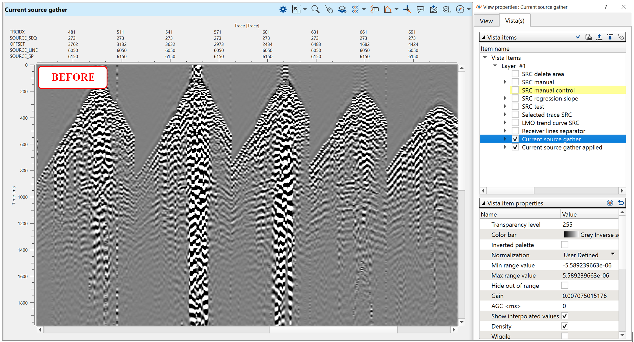
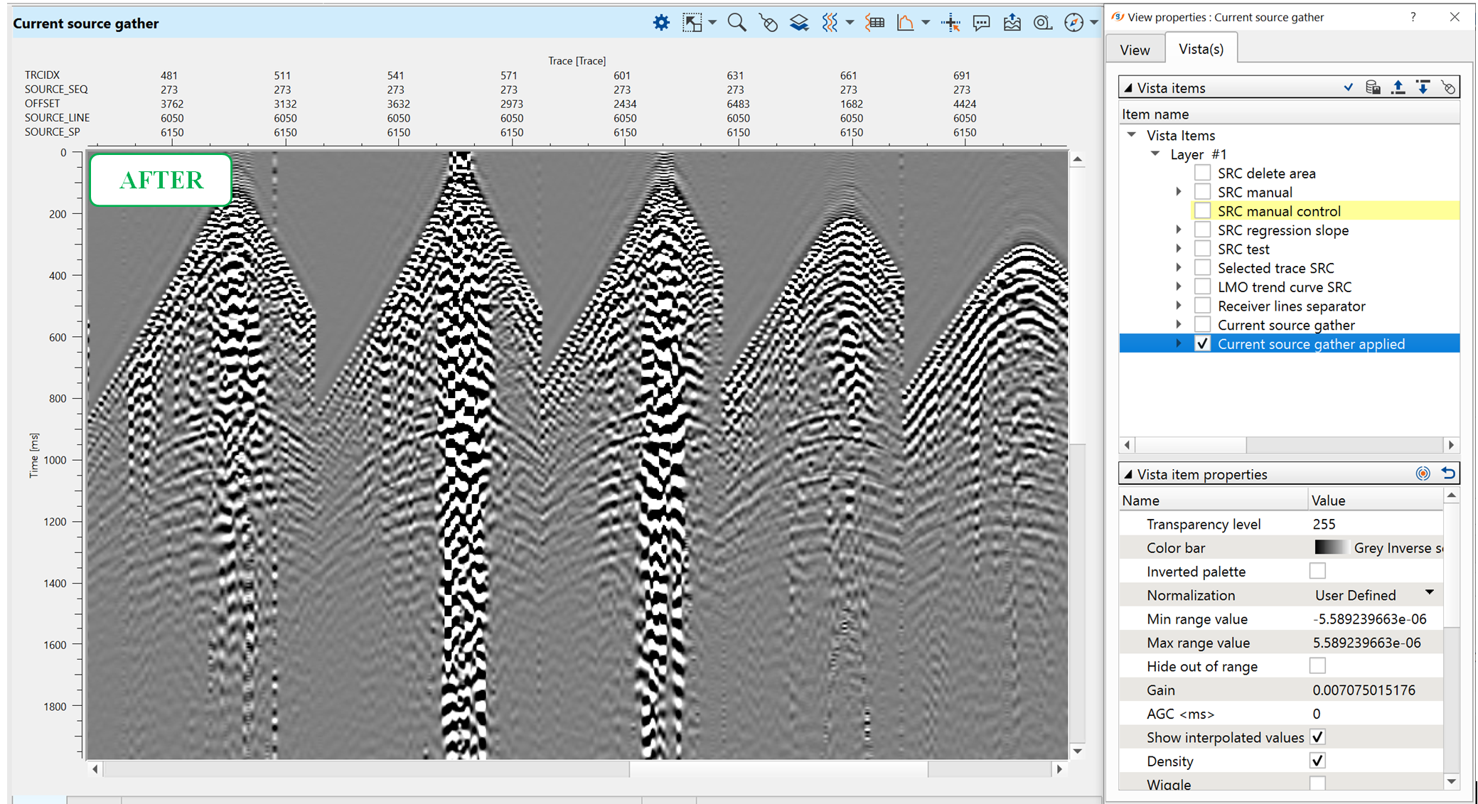
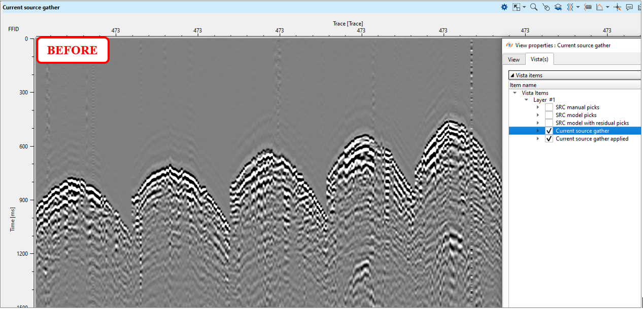
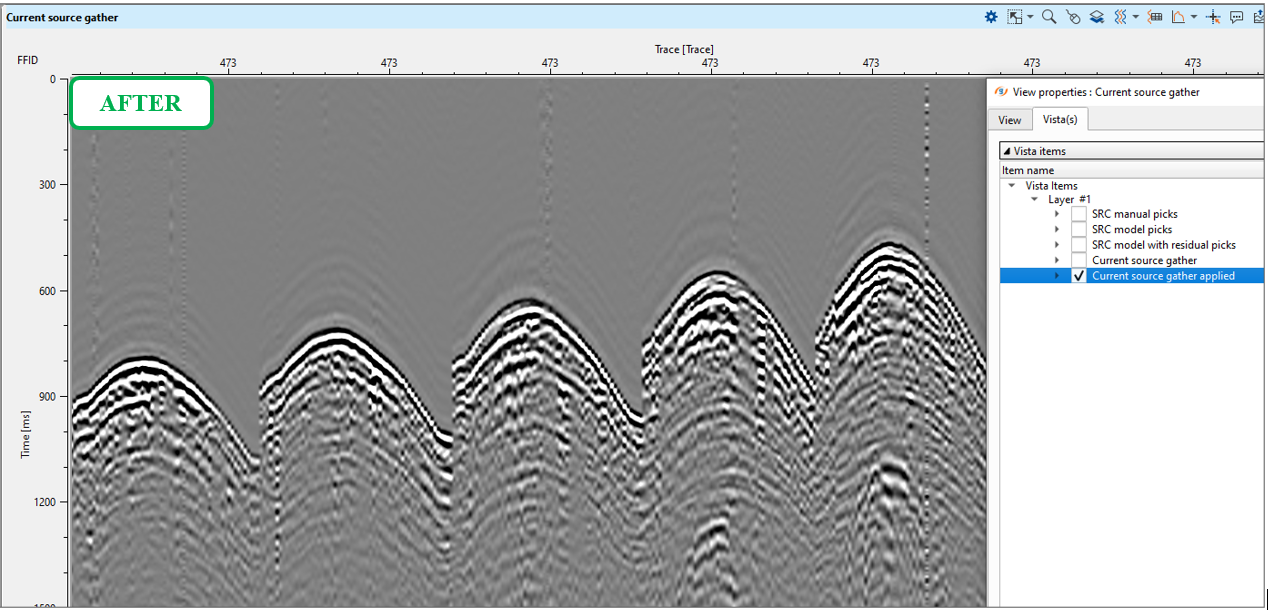
For tomography velocity view, we can define appropriate number of iteration in the parameters tab. Once the solution is computed we can do a QC of the statics result by using any of the current source/receiver gather and enable/disable the Current source gather and Current source gather applied options from the View properties of the Current source/receiver gather. Interactive fast QC by applying statics correction on gathers with different sorting: source, receiver and bin.

Check the source gather before and after statics applying. Prior to that, in the Current source gather view, we can see SRC manual picks, SRC model picks and SRC model with residual picks as shown below. SRC manual picks are nothing but the First break picks which we imported at the beginning. Based on these First break picks, it will calculate the model and residual picks.

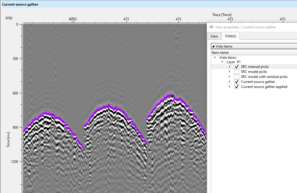
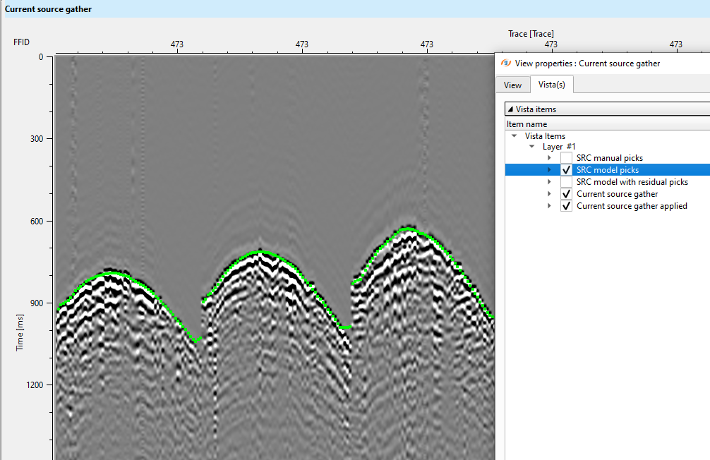
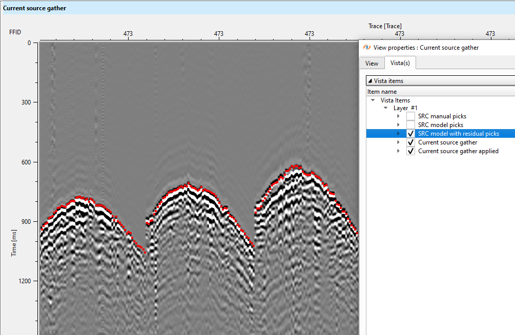
Choose any source on the Calculation area by LMB clicking and look at the source gather View Vista window and check gather before and after statics applying.

Source gather before and after tomography statics applying:

Another important QC tool is convergence graphs where you can understand how many tomography iterations should be enough. Every iteration must reduce an error/mistie between observed and modeled times. If the error is too high or the tomo convergence is not matching with the residual convergence then we need adjust the solver parameters and/or other parameters and click on the Solve option from the action item menu. It will recalculate the solution and update the displays.

Graphs of the main-tomography iteration (purple) and residual (red) solution:

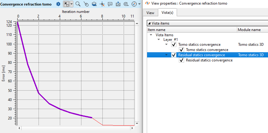
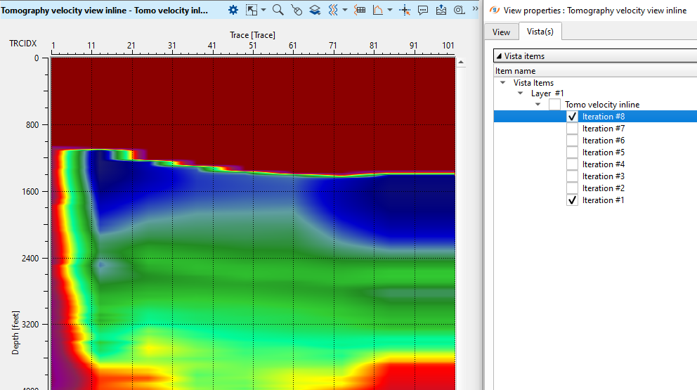
In the above image, we have 0 to 7 (total 8) iterations and the error is decreasing in accordance with iterations. Also we have 4 residual iterations. After one iteration, the error is minimal from the residual iterations. We can increase the total iterations from 8 to 15 and try to minimize the error.

Depth velocity model after tomography. Here we can observe the first iteration and last iteration (8th) and the progress in the velocity update.

Depth velocity model of the first iteration:

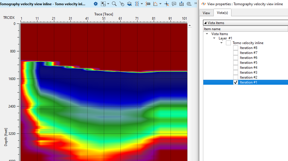
Depth velocity model of the last iteration:

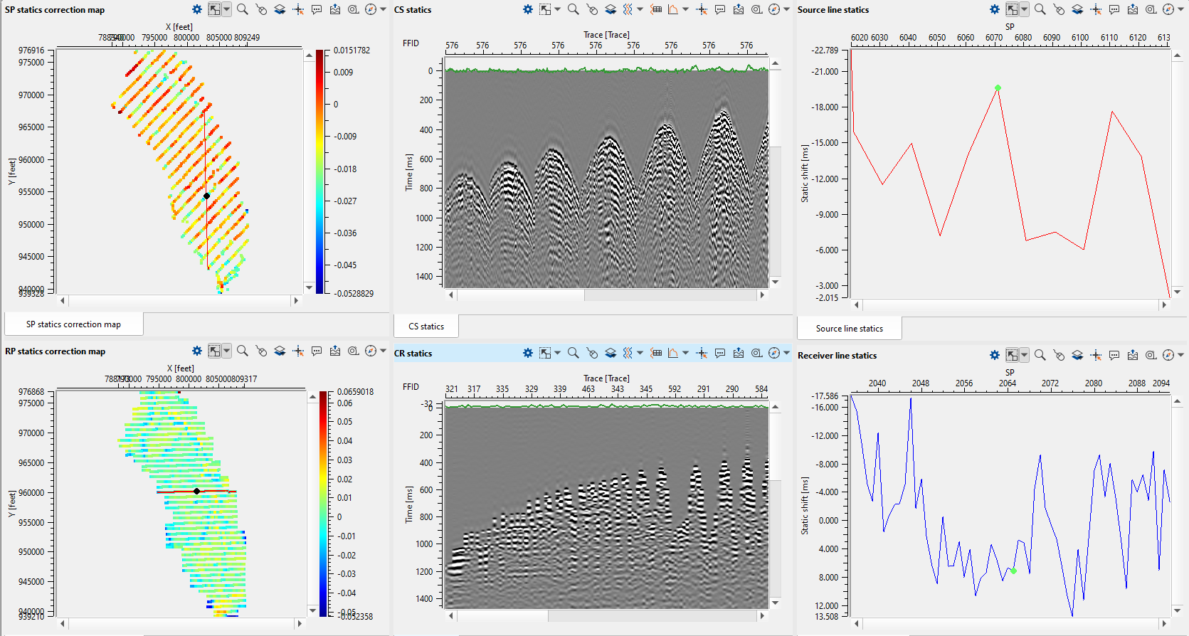
The next step is checking statics corrections by using Statics QC module (add it to the workflow):

There are few important QC Vista items (Vista Groups-> Main) like SP source, RP receiver statics corrections maps, CS, CR gathers before and after static application and Source and Receiver line statics etc.

So, we have calculated two refraction static correction: 1) conventional (regression method solving) 2) tomography. There are two ways for further step: apply static corrections to the seismic data set and save it to just save static corrections into DB (and use them later):

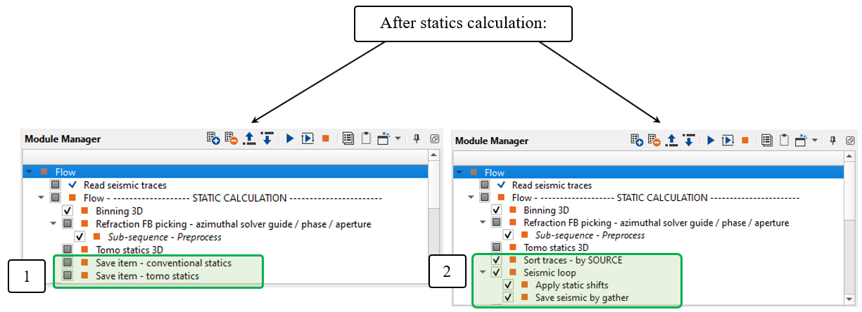
1) Save statics via Save item module:

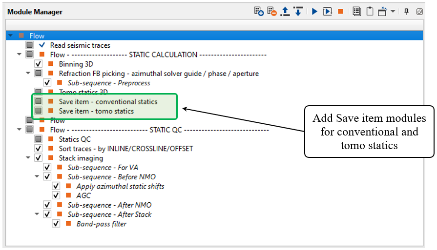
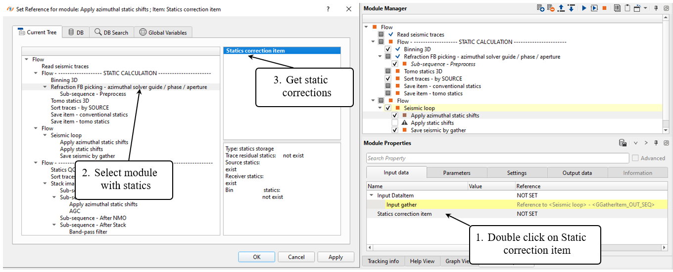
Get statics correction and connect it to the Save item modules as Item for save:

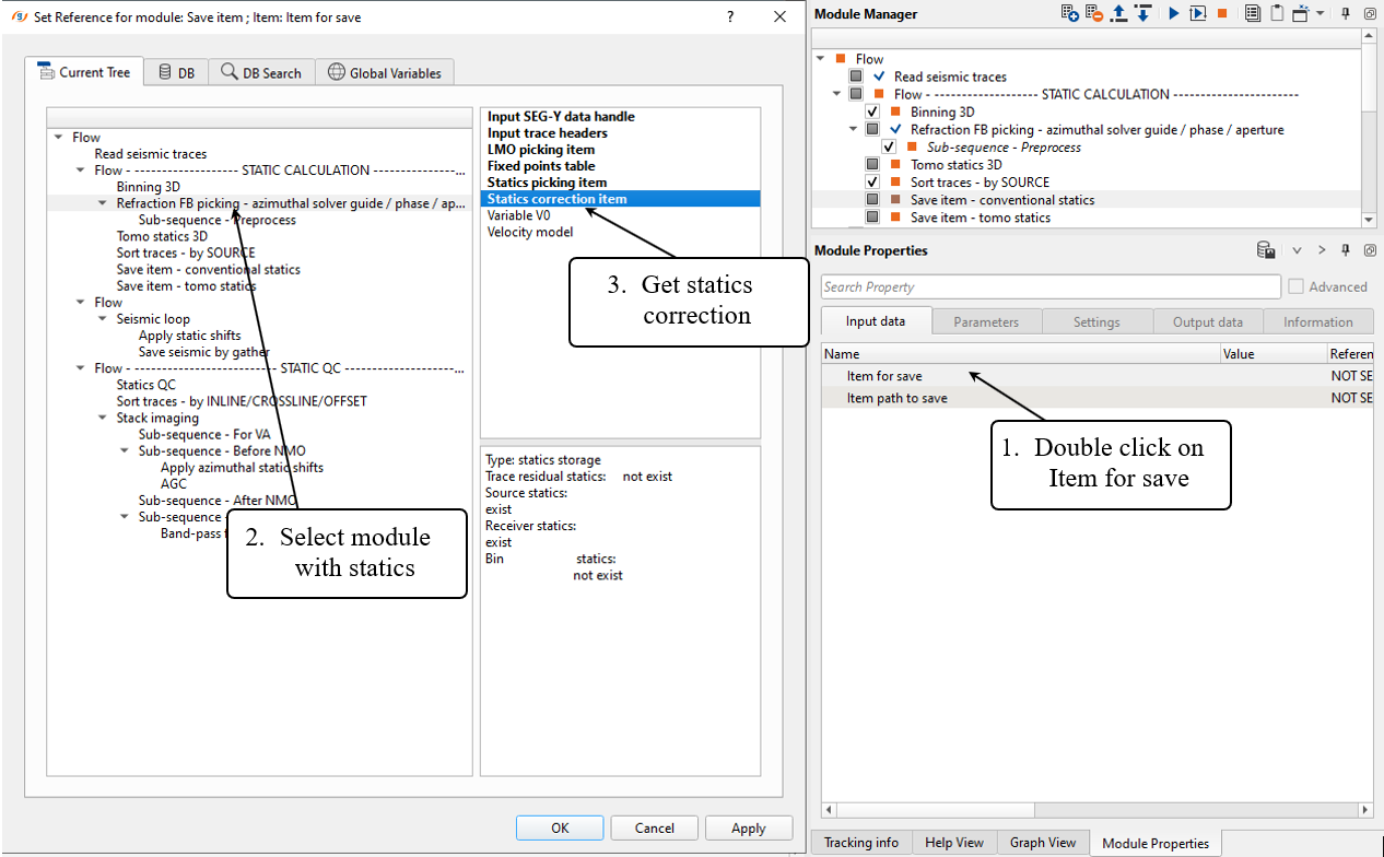
Define an output name Refr_statics_conv (in DB) of the static library:

Execute the module. Do the same for Save item - tomo statics (get statics from tomo module).

2) Apply statics and save seismic.

For saving a seismic data set with applied tomography statics corrections by using Apply Azimuthal static shifts or Apply statics shifts that work in a Seismic loop. Add all necessary modules and define a name for output data set 0040_Refraction_static_gathers, execute the seismic loop for the entire data.

                -----------------------------------------------------------------------------------------------------------------------------------

An internal data base of the g-Platform includes seismic data sets and all types of libraries.

        Library is all other types of data except the seismic, i.e. velocity, statics, muting, etc.

-----------------------------------------------------------------------------------------------------------------------------------

We can create two different dataset(s) i.e. one with azimuthal refraction statics and the other with tomography refraction statics and create the stacks to compare both results.

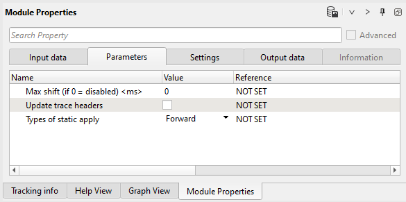
Use Apply azimuthal static shifts module for applying statics from Refraction FB picking - azimuthal solver guide / phase / aperture.

Use Apply static shifts module module for applying statics from Tomo statics 3D.

Input data for Apply azimuthal static shifts:

Parameters for Apply azimuthal static shifts:

Parameters for Save seismic by gather:

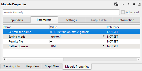
Execute seismic loop for the entire data set. Similarly, when we create the tomography refraction statics shot gathers.

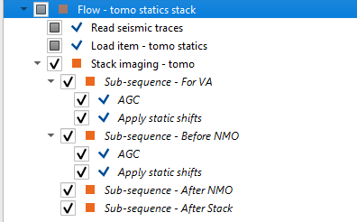
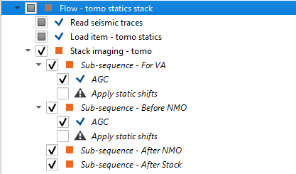
Now we can do a quick QC on a stack section. Apply refraction statics corrections to seismic traces and build a stack section via Stack imaging . Below we are displaying the workflow for creating the stacks using azimuthal refraction statics and tomography refraction statics. To create stack without any refraction statics, simply uncheck the Apply azimuthal statics shifts and/or Apply static shifts module in the workflow. We don't have to create two stacks without refractions.

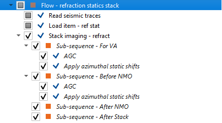
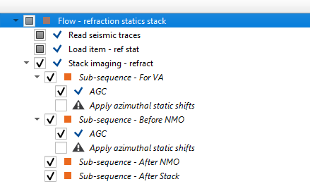
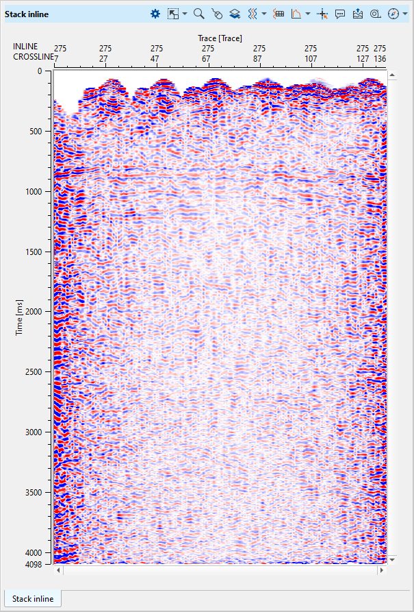
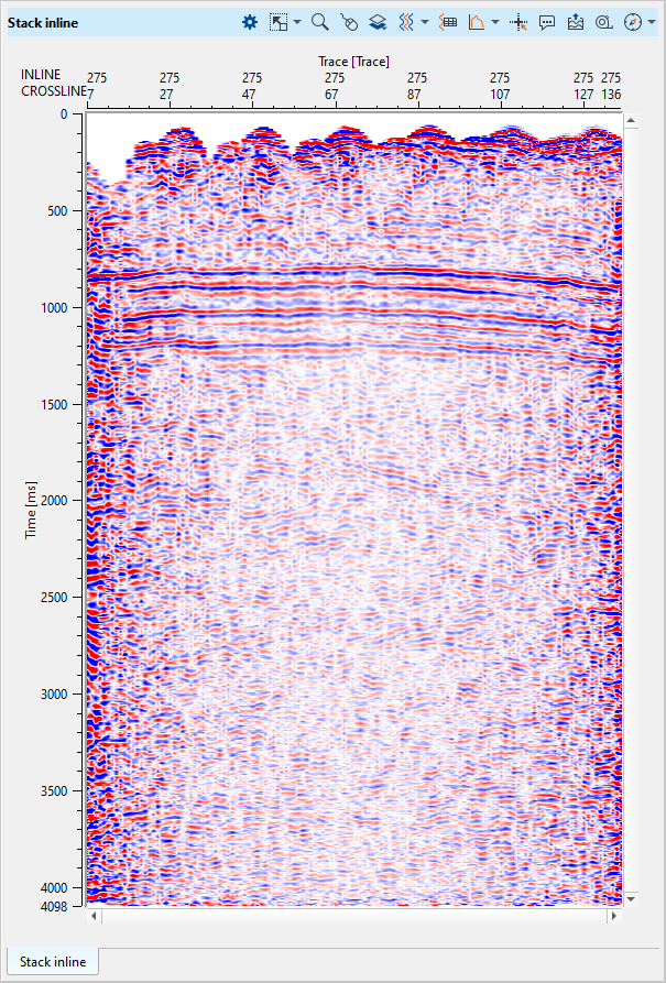
Stack section before (left) and after (right) Azimuthal Refraction statics application:

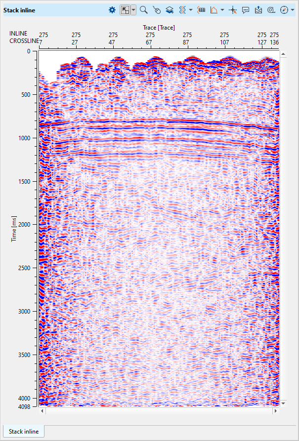
Stack section before (left) and after (right) Tomography Refraction statics application:

If you have any questions, please send an e-mail to: support@geomage.com    

First Break Picking and Refraction Statics Tutorial - Geomage g-Platform - YouTube