 | SPHERICAL DIVERGENCE |
|
<< Click to Display Table of Contents >> Navigation: Tutorials > Seismic Processing 3D LAND >
|
One of most important step of seismic processing sequence is compensation of amplitude absorption of a wavefront. For that task we can easily find Spherical divergence module. Spherical divergence correction is applied prior to pre-stack data to compensate the energy loss (amplitude decay) during the wave propagation. As the wavefront expands the energy is spread over a wider area and the amplitude decays with distance from the source. This amplitude decay is called spherical divergence.
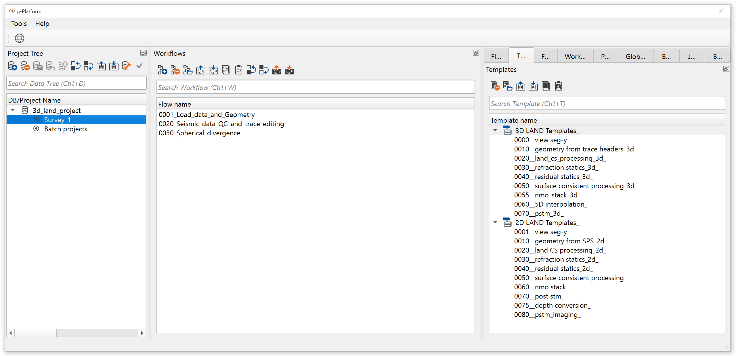
Create a new workflow 0030_Spherical_divergence.
We are going to use the following modules in this workflow:
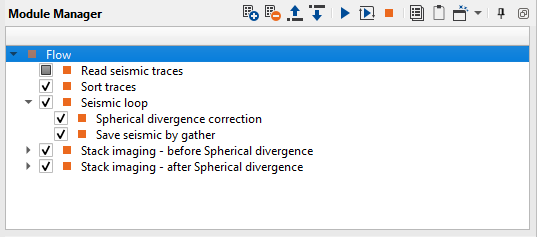
1. Read seismic traces
2. Sort traces
3. Seismic loop
4. Spherical divergence correction
5. Save seismic by gather
6. Stack imaging - before/after Spherical divergence
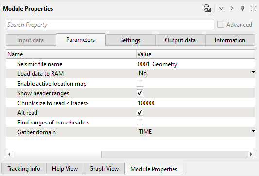
1) Read seismic traces. Define the input seismic file parameter 0001_Geometry, which is data set with geometry.
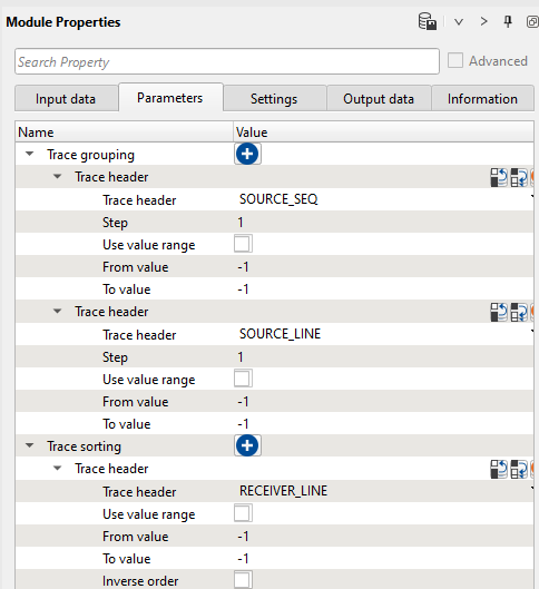
2) Sort traces. Connect the input vector with trace headers from the previous module and sort the data as SOURCE_SEQ, SOURCE_LINE in Trace Grouping and RECEIVER_LINE as Trace sorting. The user can sort the data as per their processing needs. It is required for the Seismic loop module:
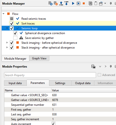
3) Seismic loop. Seismic loop is an interactive procedure designed for processing data in a gather by gather mode. Using this procedure, the user can create a sequence of specific processing modules that will be contained in the Seismic loop. Processing is performed on the seismic data based on the user specified sort order output from the Sort Traces module which must precede this module in the workflow, and must provide the sorted input trace headers. Connect input vector (Input DataItem) with trace headers and seismic data from the previous module, it automatically gets sorted headers from Sort traces and seismic traces from Read seismic traces. Launch Read seismic traces and Sort traces.
Now you execute Seismic loop by double click on it or via using launch button ![]() from the upper menu. Each run will change a source gather to the next one, or you can define any source number to jump to it:
from the upper menu. Each run will change a source gather to the next one, or you can define any source number to jump to it:
4) Spherical divergence. Put this module inside the Seismic loop and have a look to parameters:
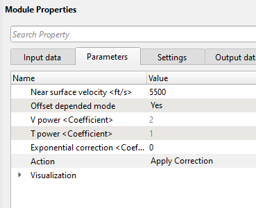
We can use single near surface velocity (V0) function or stacking (RMS) velocity field. See Input data parameter: input of velocity gather Vrms=V0 in case this parameter is not provided. Offset depended mode NO – without offset consideration, YES – offset consideration.
To compensate the amplitude decay, we need to test different combinations of spherical divergence corrections: T 2, T 2V and T 2V 2 with a single velocity function which is typically Near surface velocity.
If you choose the offset dependent (Yes option) then the equation will be offset consideration:
Coefficient (t) =(T * V 2/ V 0) * SQRT(1 + A) , where
• A = (V 2– V 0 2) * X 2/ (T 0 2* V 4), and
• X = offset of this trace,
• T = trace time at offset X,
• T 0= zero-offset time of this event,
• V = stacking velocity, extracted at time T0,
• V 0= surface velocity (extracted from vel fun at time 0), and we assume that T and T0 are related by the NMO equation:
T 2= T 0 2+ (X/V) 2
V power - if offset dependent mode is selected this option will be disabled however if the offset dependent mode is NO then the use should provide the velocity power value like 1, 0.5, 2 etc.
T power - Similar to V power, if the Offset dependent mode is selected as NO then the user should provide the T (time) power values like 0.5,1,2 etc.
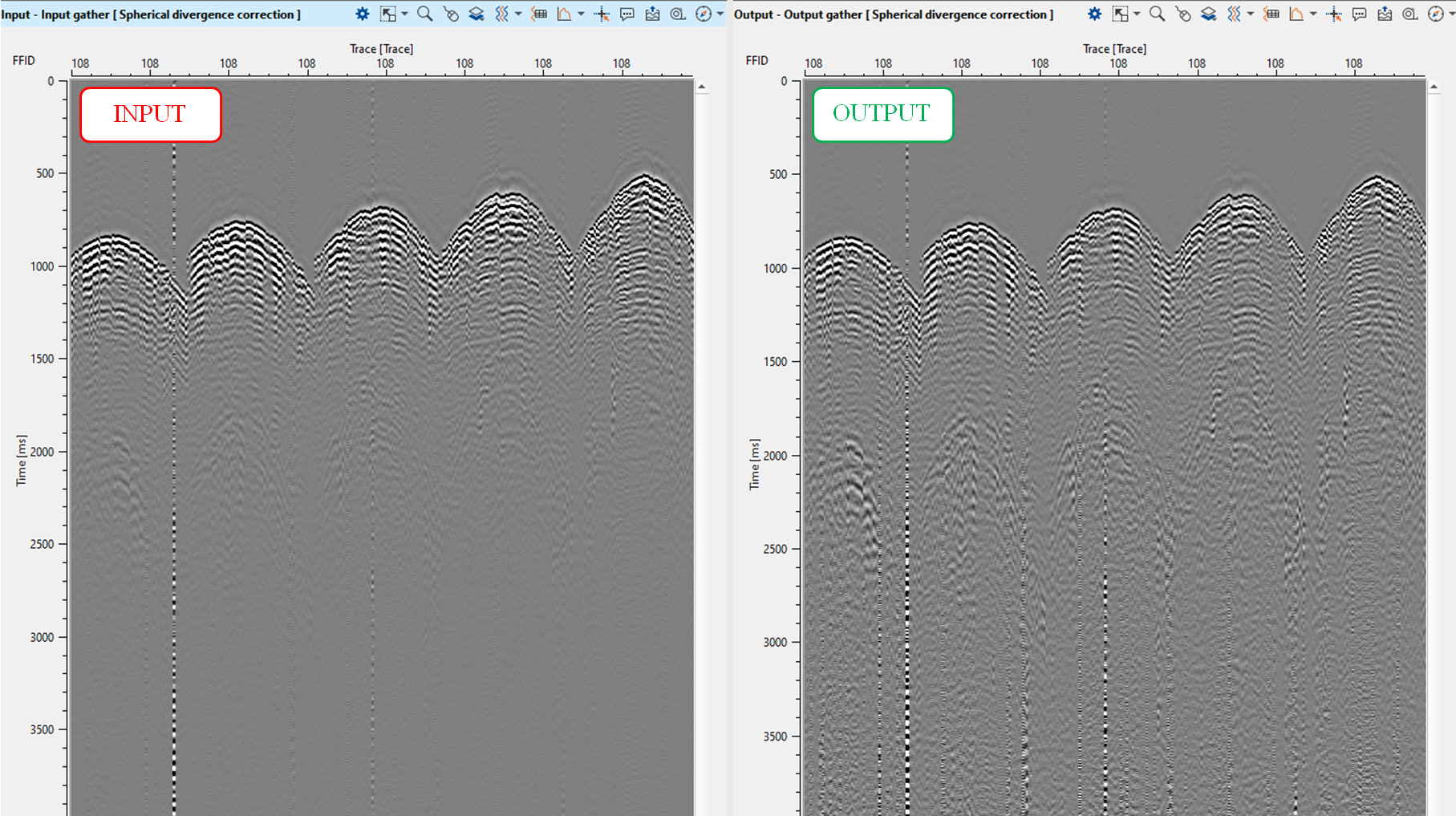
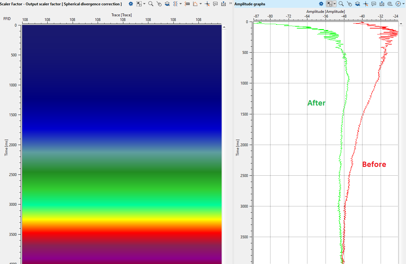
Launch Spherical divergence module add VistaGroups from Spherical divergence on your work area: press RMB on the module -> Vista Groups -> All groups -> In current window. There are four QC windows: input, output gathers; input, output amplitude graphs and amplitude coefficient (scalar factor):
On current step of seismic processing we can use single velocity function and remove before migration stage.
5) Save seismic by gather is used to save the seismic data in g-Platform’s internal format with .gsd extension. This module should be used within the Seismic Loop. Write a name of an output seismic data set 0030_Spherical_divergence and run Seismic loop on the entire data set by using launch all modules ![]() button.
button.
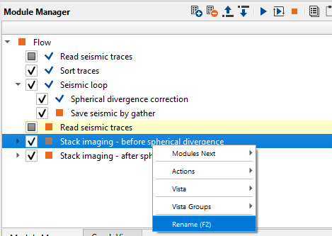
6) Stack imaging - before/after Spherical divergence. This module is a complex interactive application for velocity analysis, creating mute function, stacking CMP gathers, but we don't need to use all these option in this chapter. This step is only for QC, so we just need to build two stacks and compare them: before and after spherical divergence correction. Add Stack imaging module and write a comment: before Spherical divergence, and add the second Stack imaging with comment: after Spherical divergence:
Pay attention on what is inside Stack imaging module, it is sub-sequence. Sub-sequence helps to avoid creating a separate workflow to apply an AGC or Deconvolution or other processing modules, we just simply insert those modules in the sub-sequence inside the main module. Open sub-sequence flow in the Stack imaging module:
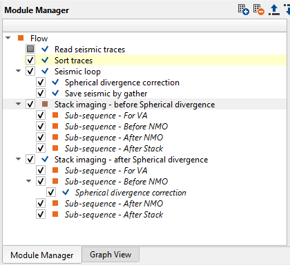
There are four sub-sequences inside Stack imaging:
•Sub-sequence - For VA: processing for velocity analysis, i.e. apply some procedures like band-pass or AGC, and then velocity spectrum is calculated;
•Sub-sequence - Before NMO: processing before applying NMO corrections to gathers, for example we can apply static corrections;
•Sub-sequence - After NMO: processing before applying NMO corrections to gathers, for example we can apply denoise procedures;
•Sub-sequence - After Stack: processing after stacking CMP gathers, for example we can apply denoise procedures or spectrum balancing.
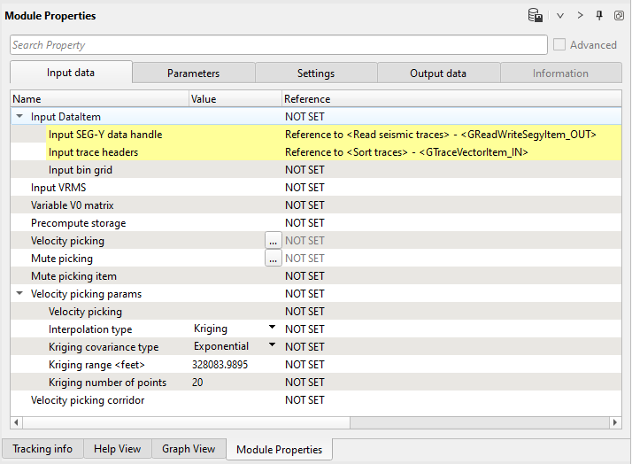
Define all necessary input data items:
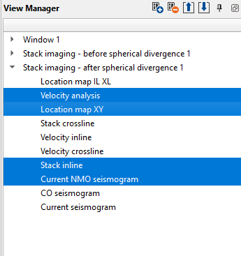
Open all Vista groups of Stack Imaging module in new window, go to the View Manager and keep the required vista items and remove unnecessary windows by either using delete button on the keyboard or right click on the vista items inside the View Manager and select Remove option:
Change windows location, refresh them by clicking on Adjust to size button. Select some CMP point from the location map by using LMB. Do not focus on velocity spectrum and picking in this chapter, because we will go deeply into velocity analysis later. For now we just need to build a stack for spherical divergence QC. Therefore, pick a single (or a few points) velocity function on the spectrum. Create a mute function using interactive Current NMO seismogram window. Use mouse for mute picking on the CMP gather:
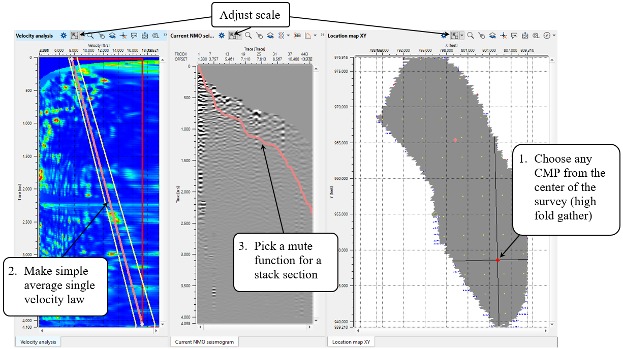
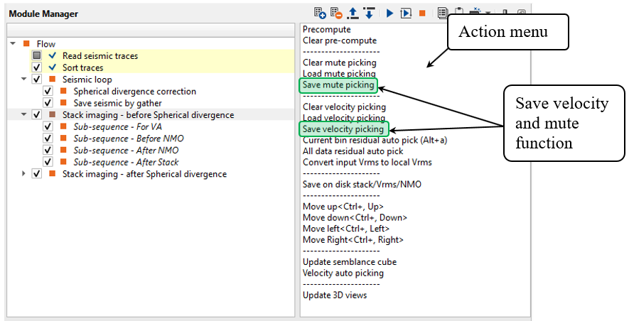
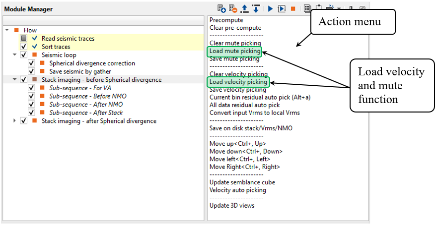
Noticed that you can save velocity and mute function on a disk via Action menu:
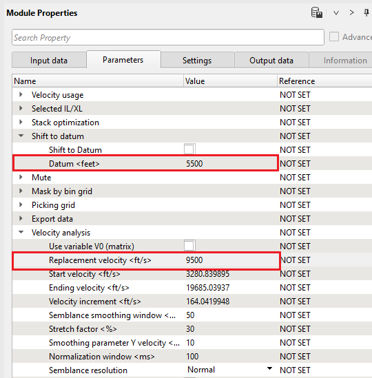
We can use default parameters just for spherical divergence QC, but pay attention that stack won't be on a constant datum. Try to compare two results: datum is on topography and datum is on constant/final. Datum plane topic will be discussed in the next chapters. For shifting seismic data from topography on constant datum you should change the following parameters:
Parameters:
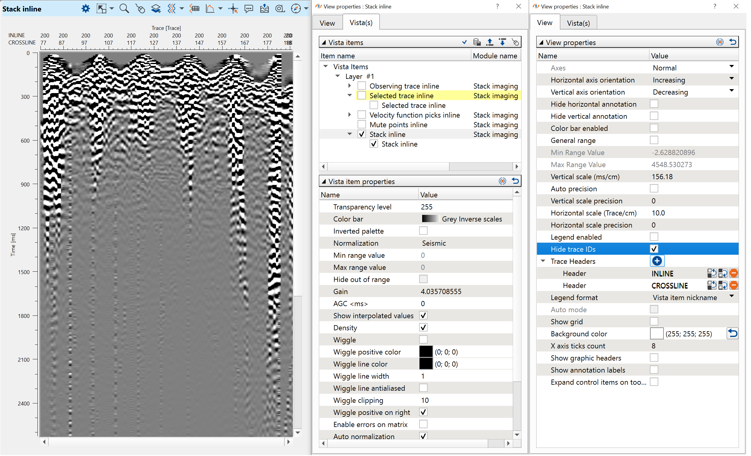
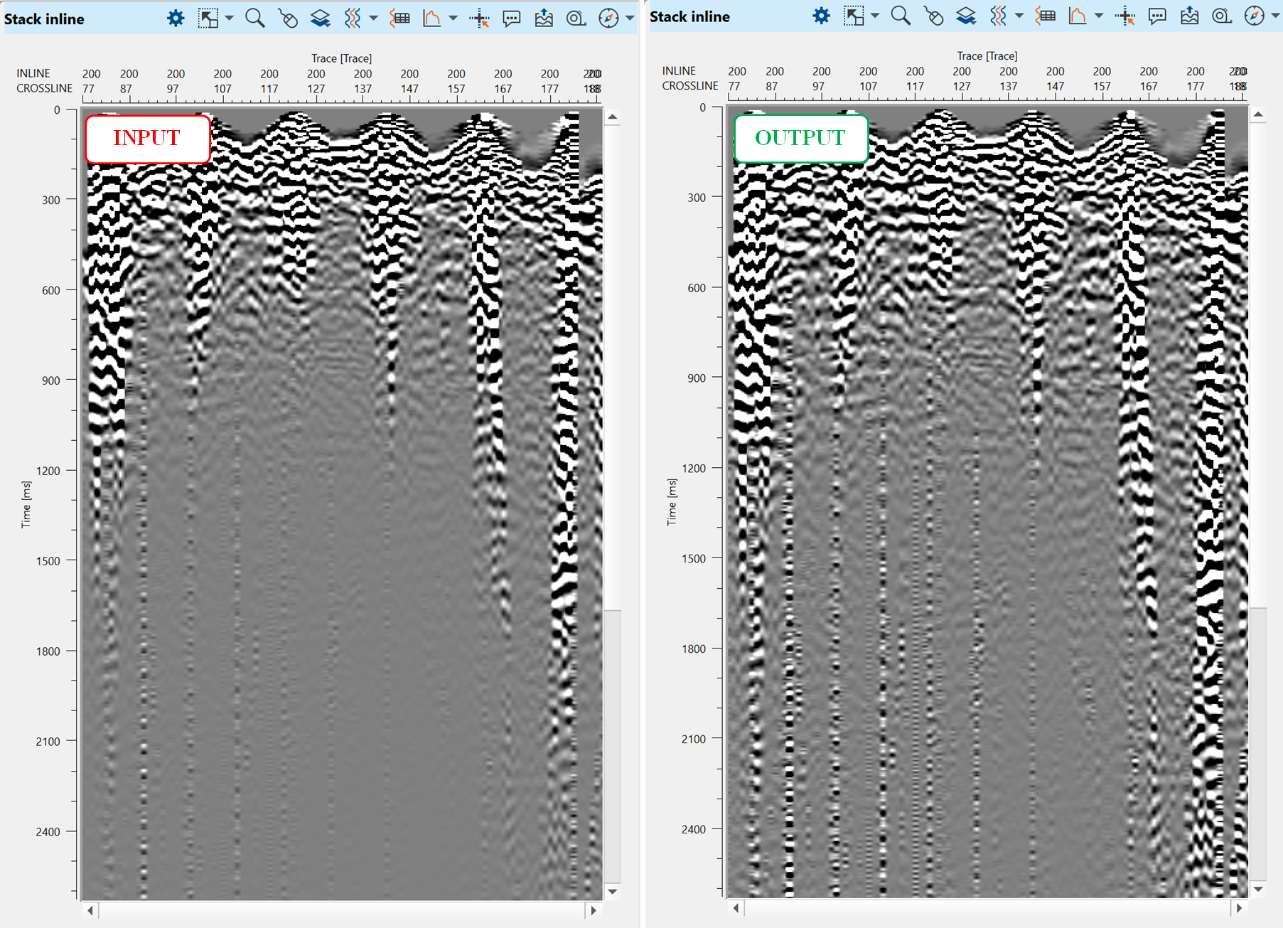
Execute Stack imaging and check result. Switch off unnecessary layers (Vista Items), this is a stack before spherical divergence:
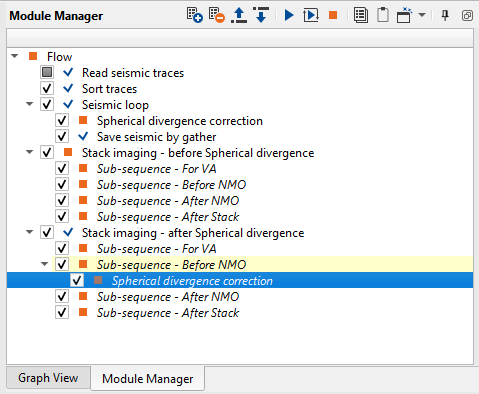
Next, we need to create the second stack after spherical divergence. Define input data items, load the same velocity and mute files, add spherical divergence module into sub-sequence and execute Stack imaging. Open two stack windows: before and after spherical divergence:
 If you have any questions, please send an e-mail to: support@geomage.com
![]() Spherical Divergence Correction and Exponential Gain - Geomage g-Platform - YouTube
Spherical Divergence Correction and Exponential Gain - Geomage g-Platform - YouTube