Residual static corrections are uniform time shifts that are applied to trace to compensate for time delays in the highly variable near-surface weathering zone. These delays occur near both sources and receivers (Wiggins et al., 1976). Residual static corrections are used for removing the short wavelength anomalies and may used in the processing land and shallow marine data. The application of residual corrections improves the final seismic section more than when only datum statics applied (Cox, 1999). Input seismic data must be a moveout-corrected CMP gathers. For this task we are going to use Surface-consistent residual static correction module.

At the initial stages of the pre-processing, the poor signal to noise ratio (SNR) of CMP stack quality is due to the near surface velocity anomalies and topographic changes of the surface. These changes give rise to travel time shifts and it can be corrected by using various methods like refraction statics by means of picking first breaks and calculate the statics and apply them. Second method is Surface Consistent Residual Statics.

Create a new workflow 0090_Residual_static_correction:

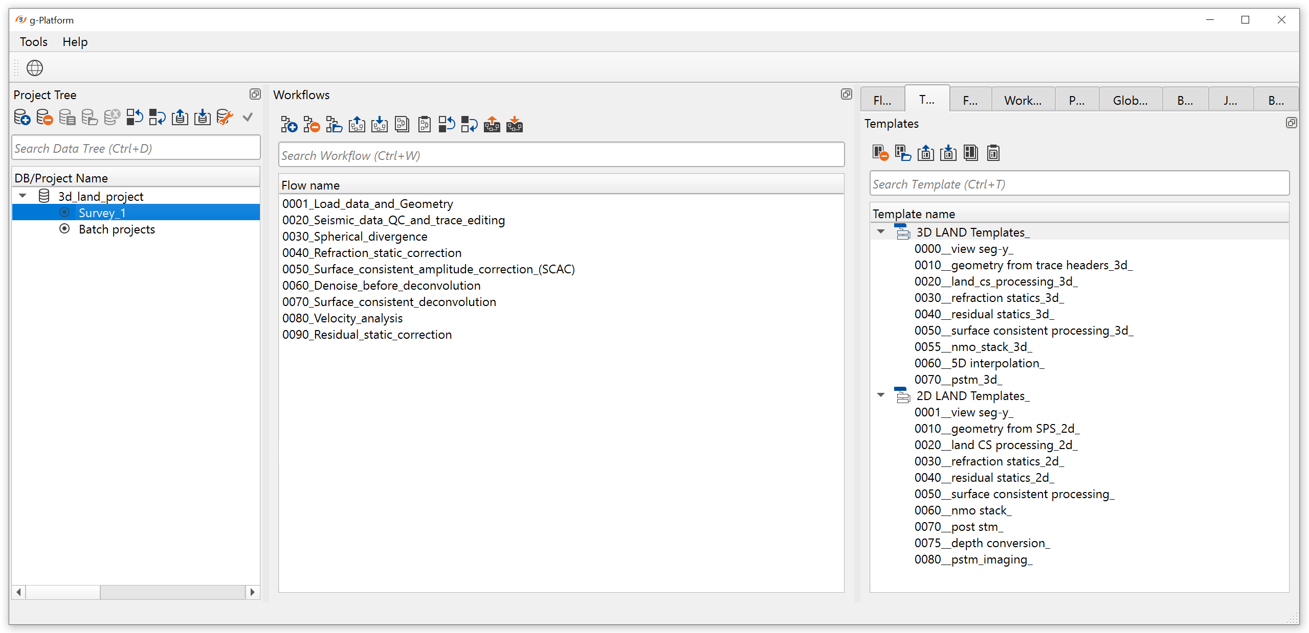
Open the workflow and add all necessary modules as shown below:

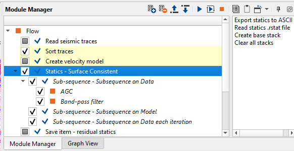
1) Read seismic traces: load 0060_SCDecon seismic data set.

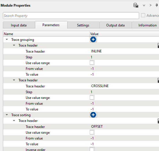
2) Sort traces: perform a Inline/Crossline - Offset sorting for residual static calculations.

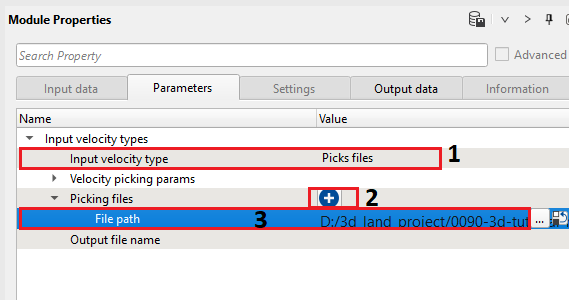
3) Create velocity model: Create the velocity model by selecting the Input velocity type as Picks file. Next, click on icon and browse through the folder to provide the input velocity file.

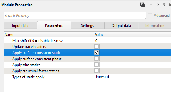
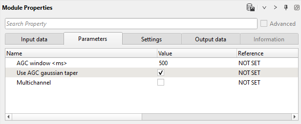
4) Statics - Surface Consistent: Define all input data parameters. Add AGC and Band-Pass filter. It provides opportunity to apply any processing procedures before calculation of residual static, i.e. we need to prepare input seismic data for residual statics: automatic gain control and band-pass filtering as shown below. Notice that we already applied refraction statics.

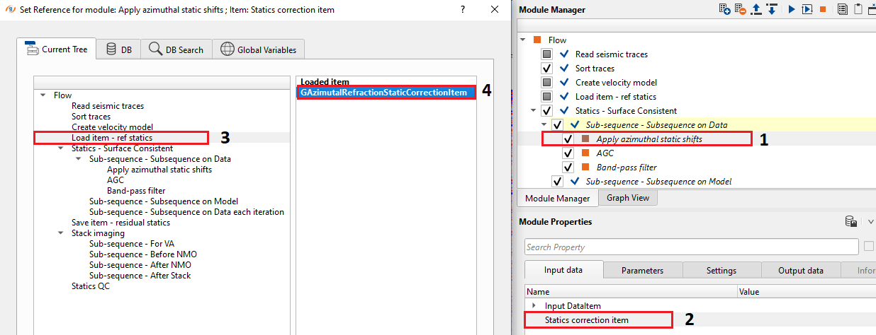
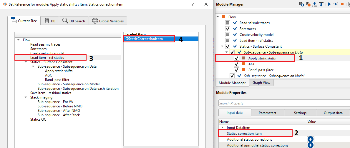
In case we didn't prepare the input data with refraction statics, we can add the Apply azimuthal refraction statics module (in case of using Refraction FB picking - Azimuthal solver guide/phase/aperture) module and Apply static shifts module (Tomo statics 3D).

Apply azimuthal statics shifts

Apply static shifts

Select the appropriate option(s) from the Parameters.

AGC:

Band-pass filter:

Statics - Surface Consistent:

In the Surface Consistent Statics, it computes single static solution for all the traces that is coming from the same shot gather. In the case of receiver, separate statics corrections are applied for all the traces from the same receiver. For the combined statics correction, each trace coming from single shot and single receiver will have separate shot static and separate receiver statics. Combining these source and receiver statics give rise to single time shift or static correction.

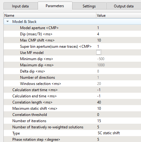
In g-Platform, module Statics – Surface Consistent builds the pilot trace from the CMP stack based on the Model aperture (CMP) defined by the user at the Model & Stack Parametrization. For example if user input the Model aperture (CMP) as 1, it means there will be 3 traces for generating the model trace. There is one trace on the left of the center trace and one on the right side. As a first step, the center trace is cross correlated with the traces on both side of it and generates a model trace and stores in the memory and the process follows to the next trace and so on till to the last trace.

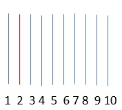
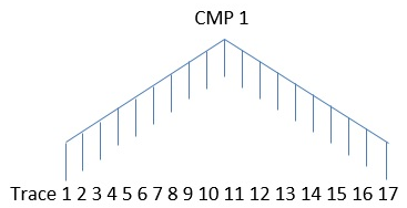
In the above image, red trace acts as center trace and it do the cross correlation with the adjacent traces and generates the model trace. In the second stage of the surface consistent statics calculation, this model trace calculates the shift for the pre-stack gather of the CMP by means of cross correlating with the each individual trace.

In the final step, we are solving the equations using Gauss Seidel in an iterative way to get the shifts for each individual shot and receiver gathers. Within this module, we have Velocity Update parameter where in user can enable Velocity updates to automatically update the velocities with each iteration.

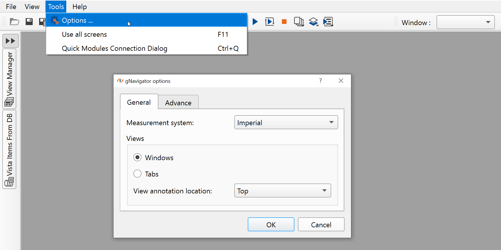
Originally, Teapot 3D data has imperial measure system, so you can change it in g-Navigator:

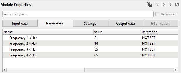
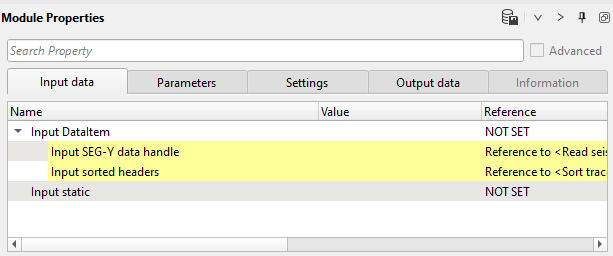
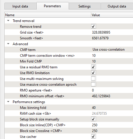
Define all necessary parameters as shown below:

Input data:

Parameters:

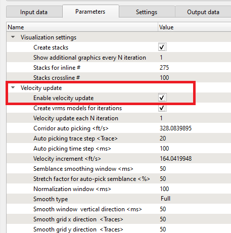
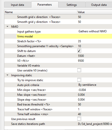
We have an option for updating velocity model by using the enable velocity update option (as shown in the above image). In this exercise, an algorithm updates the velocity model for displaying the results with updated velocity model. The input seismic gathers are not NMO-corrected, so we need to apply stacking velocity inside the module. Therefore, we have to define Vrms model parameter:

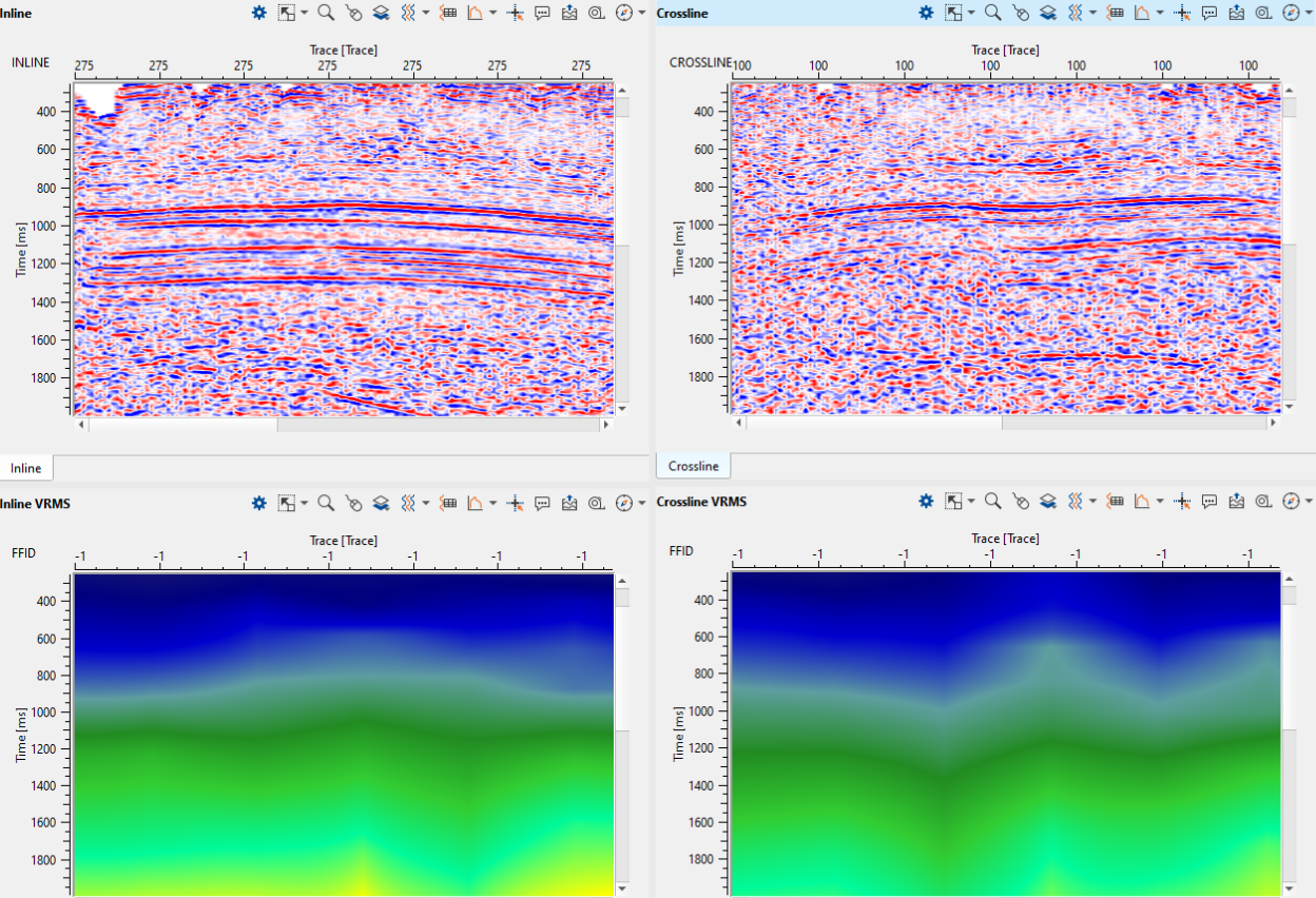
Other parameters are remain unchanged (by default). Execute residual statics and check results, open all visual vista views: Stacks for defined (in parameters) inline and crossline, as well velocity model:

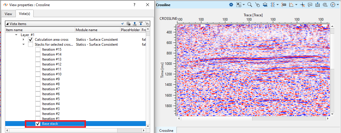
How to check stacks before and after residual statics: module calculates stacks automatically for each iteration: in the below image, we can see the Crossline stack before residual statics applied which is represented as a Base stack with the provided input velocities.

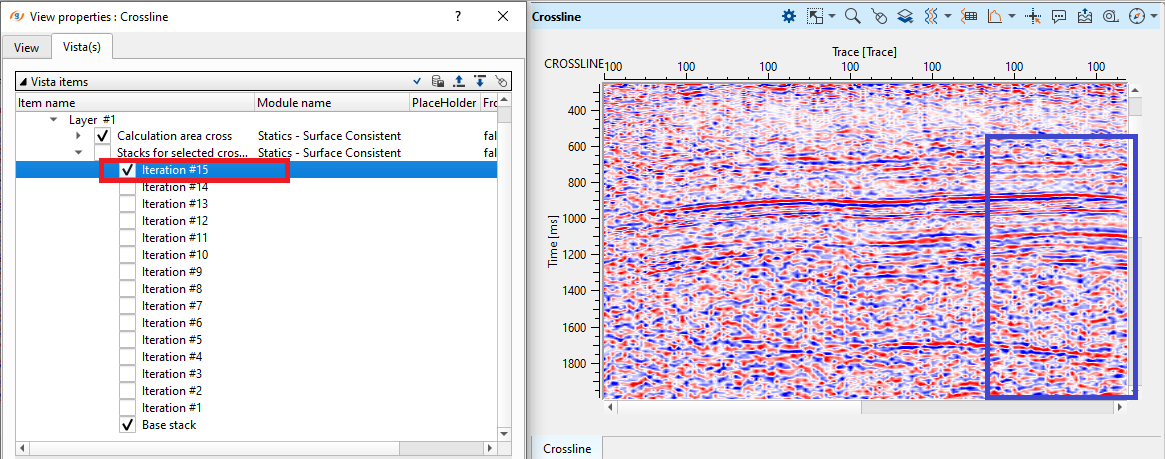
After 15th iteration with corresponding velocity updates, look at the stack response of Crossline with the application of residual statics.

We can run multiple passes of residual statics with different parameters (window, iteration, length of correlation, max.shift statics, etc.) and to get better residual static solution.

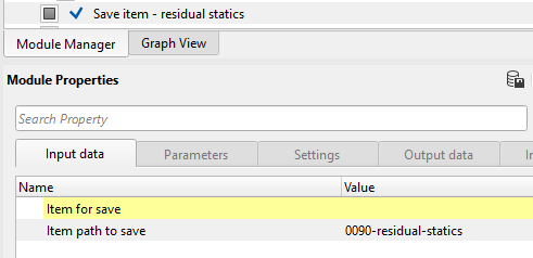
6) Save item: When you satisfied with the result save residual static corrections to DB via Save item module:

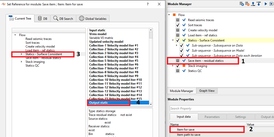
And define an output name for residual static library, write 0090_Residual_statics and execute the module. Similarly, we can save updated velocity model also.

Now we can use residual static correction in other workflows. In case we need to read the particular iteration like iteration 5 out of iteration 15, then we can select Read statics .rstat file option from the action menu. It will open a file explorer window. Browse the file and select the particular statics file.

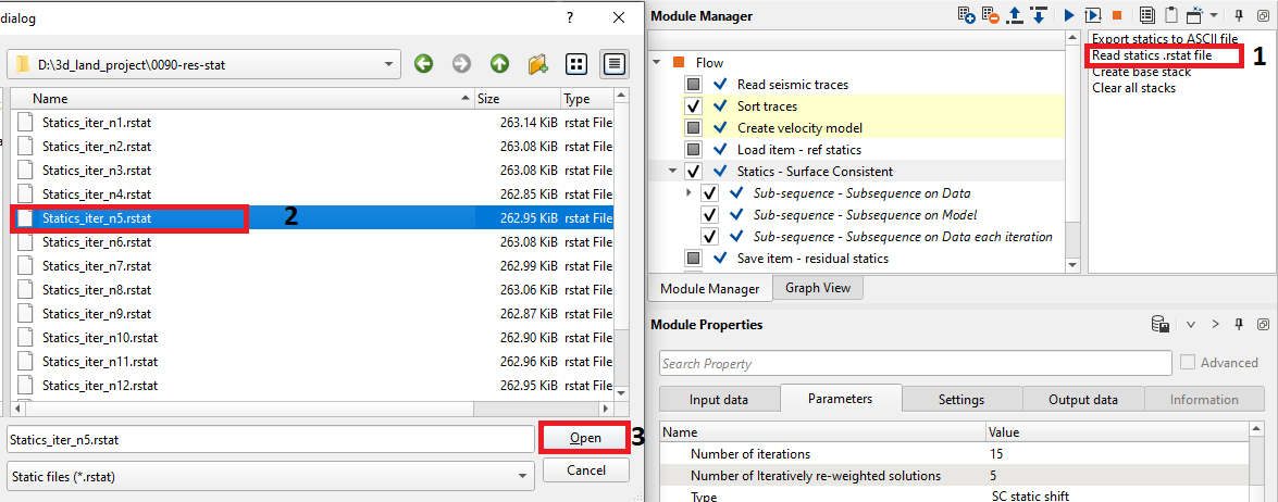
In the same way, we can save the residual statics by selecting the Export statics to ASCII file option from the action menu.

-----------------------------------------------------------------------------------------------------------------------------------------------------------------------------------------------------------------------------

Please make a note that, whenever we wants to change the parameters and rerun the Statics - Surface consistent module, we MUST clear all the previously calculated stacks by clicking Clear all stacks option from the action menu. Otherwise, it will continue creating the stacks however the numbering will be different. For example, in the first run  we created stacks with 15 iterations. Later, we changed few parameters and execute the module without clearing the stacks. So the new stacks will start from iteration 16 (as base stack since previous 15 iterations along with the base stack are still existing) followed by other iterations. The final iteration will be 31 (in case we put 15 iterations in the second execution also). 

-----------------------------------------------------------------------------------------------------------------------------------------------------------------------------------------------------------------------------

If you have any questions, please send an e-mail to: support@geomage.com  

Surface Consistent Residual Statics - Geomage g-Platform - YouTube