3D grids are essential tools used to organize and visualize subsurface data in a structured format. The process typically involves the interpolation of scattered data points (e.g., well tops or seismic picks) across a predefined grid.
Grids are built using interpolation techniques that estimate unknown values between data points. The grid can vary in resolution, based on the interpolation steps defined by the user, allowing flexibility in adapting to different geological complexities.
To begin the 3D gridding process in g-Space navigate to the Data Manager, find the 3D Grids section. This is where grid data will be organized and stored.
To create a new grid right-click on the 3D Grids folder and select Create Grid, then name it in the pop-up window. This will open the grid creation panel.
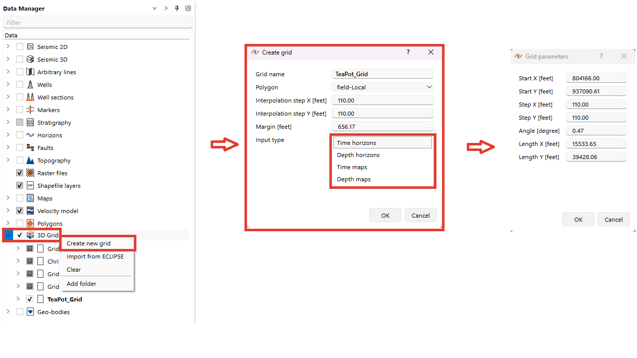
In the grid creation window, you will define key parameters that influence the resolution and extent of the grid.
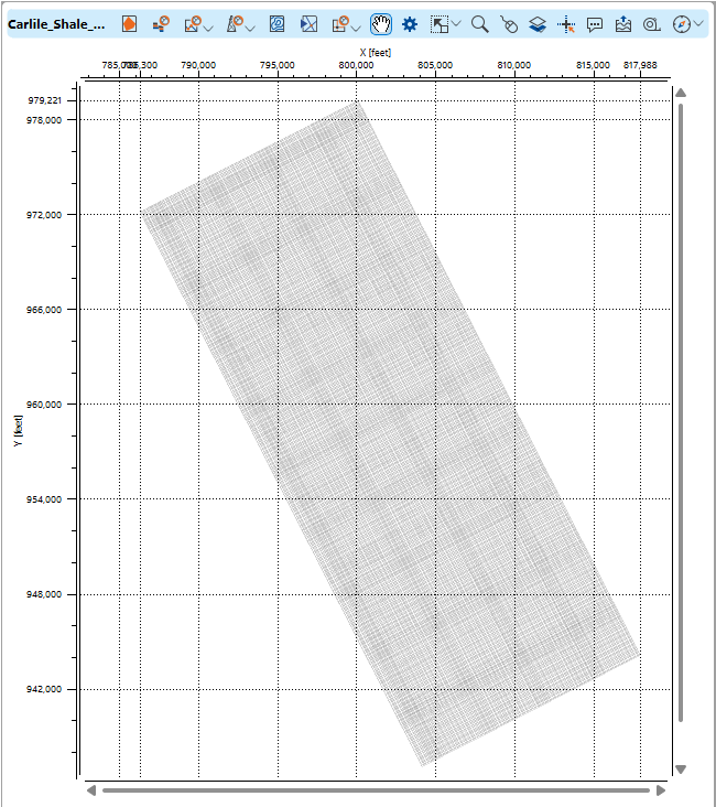
•Polygon: If available, you can select a polygon to limit the grid to a particular area. Choose “Not required” if the grid is intended to cover the full extent of the data.
•Interpolation Step X [ft/m] and Interpolation Step Y [ft/m] These define the resolution of the interpolated data. Smaller steps result in higher grid resolution, capturing finer geological details but increasing computational demand. Larger steps provide a more generalized view but are faster to compute.
Notes
Geological Context: In regions where fine stratigraphic details or thin reservoirs are critical (e.g., offshore channels, thin carbonate layers), smaller steps (10-20 ft/1-5 m) may be appropriate. In contrast, for larger, homogenous geological structures (e.g., broad anticlines or synclines), larger steps (50-100 ft/20-50 m) may suffice.
•Margin [ft/m]: This parameter sets an additional boundary around the grid. A larger margin might be useful in areas where you expect the geology to extend beyond known data points.
•
Click OK to proceed to the next step, where you define the grid parameters.
After defining the interpolation settings, you will be prompted with the Grid Parameters window (as shown in the image above). This window controls the structure and size of the physical grid.
•Start X [ft/m] and Start Y [ft/m]: These values define the starting coordinates of the grid in the X and Y directions.
•Step X [ft/m] and Step Y [ft/m]: These values determine the spacing between the grid nodes along the X and Y axes. Smaller grid steps result in a finer grid, while larger grid steps produce a coarser, more general representation.
Notes
Geological Context: For detailed geological structures, use smaller grid steps (e.g., 10-20 ft/1-5 m). Larger grid steps (e.g., 50-100 ft/20-50 m) can be used for large-scale structural features.
•Angle [degree]: This defines the rotation of the grid relative to the coordinate system.
Notes
Grid rotation is essential for aligning the grid with key features to improve accuracy and efficiency:
1.Tectonic Structure Alignment: Rotate the grid to match elongated tectonic features, minimizing the number of cells inside the reservoir contour while preserving horizontal resolution.
2.Well Patterns: Aligning the grid with injection and production wells ensures more direct fluid flow paths, reducing filtration time and increasing efficiency.
3.Fault Orientation: Rotating the grid along fault trends prevents grid distortion near faults, maintaining smooth geological transitions.
•Length X [ft/m] and Length Y [ft/m]: These define the total dimensions of the grid, controlling how far the grid will extend in the X and Y directions. Adjust these based on the size of your study area.
Once these parameters are set, click OK to generate the 3D grid.
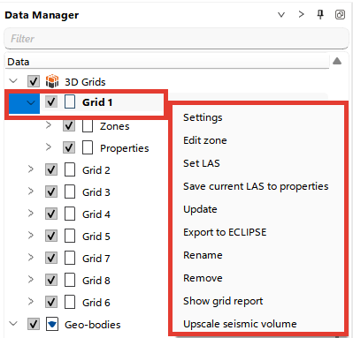
In this menu from the 3D Grid section of the Data Manager, various options are available for working with a specific grid (in this case, named "TeaPot_Grid"). Here is a breakdown of each option:
Settings: Opens the settings window where the user can modify grid parameters, such as interpolation and grid steps, margins, and other key parameters related to the grid structure.
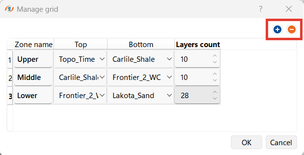
Edit zone: Allows the user to modify or create zones within the grid. Zones represent specific regions of interest within the grid that may have different geological properties or require separate analysis. Using the top buttons + and - the user can add and remove zones, and adjust the number of layers in them on the grid manager panel
Notes
The number of layers in a zone, is influenced by several factors:
1.Geological Heterogeneity: The vertical variability in properties, like the average thickness of reservoir layers, dictates layer thickness. For instance, if the average layer thickness is 1 meter, grid cells larger than 50 cm shouldn't be used to capture details effectively. This is assessed using histograms of layer thickness.
2.Well Data Sampling Interval: Typically, well data is sampled at intervals of 0.2 to 0.4 meters, which affects layer thickness.
3.Total Thickness: The entire thickness of the interval to be subdivided impacts the number of vertical layers required.
4.Computer Limitations: The computational power available may restrict the grid resolution that can be practically implemented.
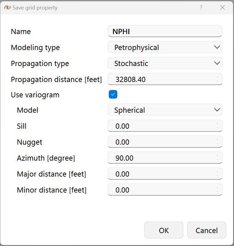
Set LAS: This option is used to assign a LAS file (Log ASCII Standard) to the grid, enabling integration of well log data for further interpretation or visualization.
Save current LAS to properties: Saves the LAS data currently assigned to the grid as a property, which can be used for various geological calculations and further analysis.
Update: Refreshes or recalculates the grid, applying any recent changes in data or grid parameters.
Export to ECLIPSE: Allows the user to export the grid to the ECLIPSE format, which is widely used for reservoir simulation and modeling. This function is critical for taking the grid data from g-Space into reservoir simulation software.
Rename: Renames the selected grid in the Data Manager for organizational purposes.
Remove: Deletes the selected grid from the project.
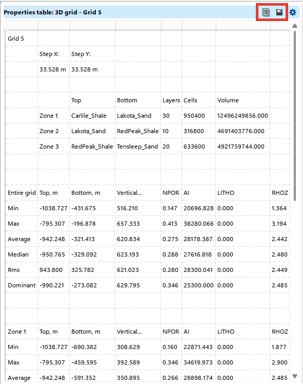
Show grid report: Opens a table displaying general parameters of the grid, such as dimensions, resolution, and volume. Additionally, the report provides detailed information for each zone within the grid. The data from the grid report can be copied directly or saved as a .CSV file
Upscale seismic volume: Allows the user to integrate seismic data into the grid by upscaling a seismic volume. The user selects a seismic volume and defines modeling parameters in a pop-up wizard. This process involves resampling the seismic data to match the grid resolution, enabling the use of seismic attributes in property modeling and reservoir analysis.
Advanced Options and Applications
Polygon Clipping: If you are working in a specific region of interest, using a polygon to limit the grid’s extent can reduce computation time and ensure focus on relevant data.
Time vs. Depth Grids: Grids can be created in both time and depth domains. Time grids are typically based on seismic data, while depth grids incorporate well data and velocity models for more accurate geological interpretations.
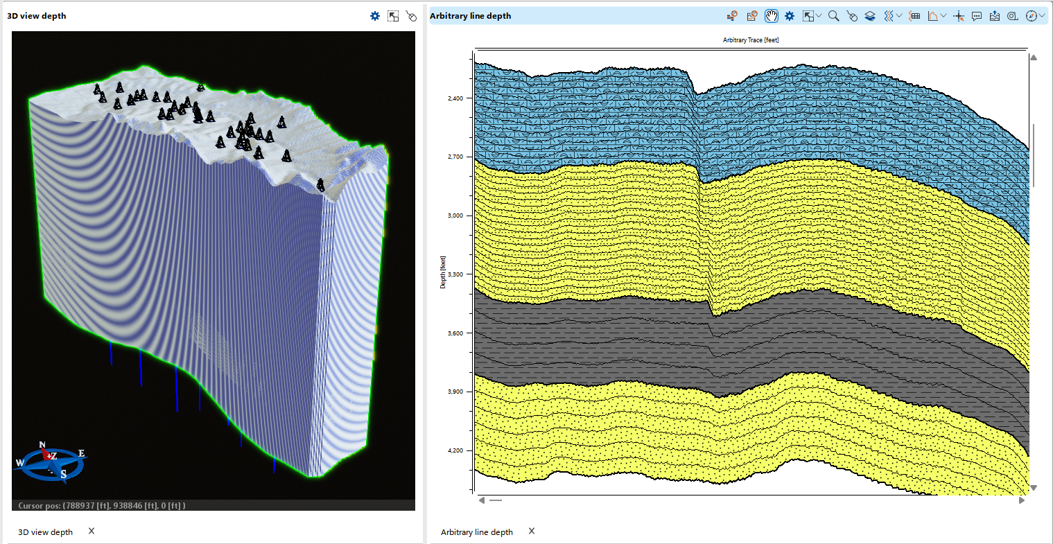
3D grid can be visualized in 3D depth view as well as in section view. Visualization settings can be configured in the Visual Settings, in the example below, lithological fill type is selected for the Grid zones.