In g-Space, Properties modeling involves the integration and calculation of well log data and other geological properties to populate 3D grids with meaningful information, such as porosity, permeability, and fluid saturation.

To start, navigate to the Data Manager, Select the desired grid (e.g., "Grid 1") by clicking on it.  This action highlights the grid and makes it the active selection.

Right-click on the selected grid to open the context menu. This menu contains various options related to the selected grid, allowing for efficient data management.

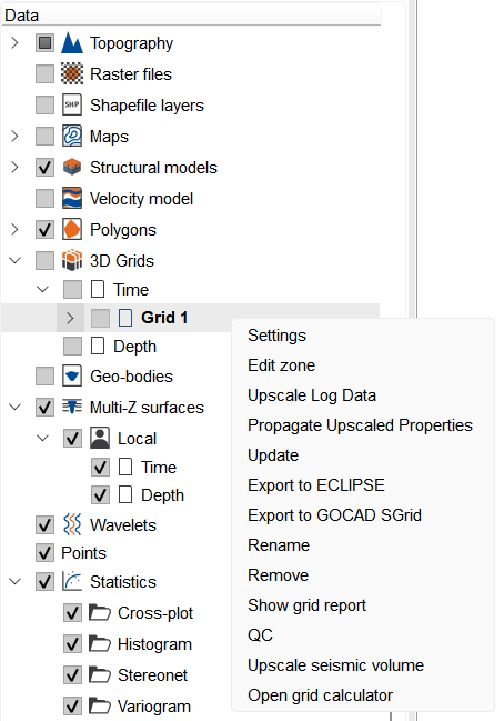
Upscale Log Data blocks (upscales) the selected well log curve onto every 3D grid cell that a wellbore trajectory crosses, averaging the log samples that fall inside each cell. Only cells crossed by a well receive a value; all other cells stay empty, so you can QC the conditioning data before property modelling. The LOG upscaling parameters window will appear, where you choose the wells, the LAS curve and how the samples are averaged.

1. LAS Curve Selection: The user can select the type of curve from the dropdown, e.g., DT (Sonic), GR (Gamma Ray), etc.

2. Averaging method: dropdown offers multiple statistical methods to extract well log data into the grid:

• Average: Computes the length-weighted average of the log samples that fall in the cell. Each sample is weighted by the length of well trajectory it represents inside the cell (the sum of value × segment length divided by the sum of segment lengths), so uneven sample spacing and trajectory angle do not bias the cell value.
• RMS: Extracts the Root Mean Square value, providing a weighted average of the data, emphasizing higher values.
• Minimum: Selects the minimum value of the LAS curve in the given interval.
• Maximum: Extracts the highest value of the LAS curve in the interval.
• Most common: Identifies the most frequent or significant value within the LAS data.
• Median: Extracts the median, giving the middle value of the LAS curve data, minimizing the impact of extreme values.

3. Curve type: select Continuous or Discrete. The type is auto-detected from the LAS curve and can be overridden. It filters the Averaging method above: continuous curves offer Average, RMS, Minimum, Maximum and Median; discrete curves offer Most common and Percentage. Choosing Percentage reveals a Facies code field; the cell value is then the fraction of the in-cell trajectory where the curve equals that code (0–1).

4. Min cutoff / Max cutoff: samples below Min cutoff or above Max cutoff are discarded before averaging; a sample exactly on a bound is kept. Both fields open on the data range of the selected LAS curve — the lowest and highest valid values it holds across the wells currently selected, ignoring null and invalid samples — rounded outward so an automatic cutoff never clips a real sample, and shown with two to six decimals according to the size of those values, so a small-range curve is displayed more precisely. They are recalculated the same way whenever Wells, Folder, Filter, Selected wells or LAS curve changes, replacing whatever the fields held, but they stay editable and keep a value you type until one of those selections changes again. A stored pair whose Min cutoff is lower than its Max cutoff, for example from a saved workflow step or an earlier run, reopens unchanged. If the selected curve has no valid values in the selected wells, both fields are set to 0.00 and the Min cutoff and Max cutoff labels turn red, with the tooltip "Selected log has no valid values in the selected wells". Equal bounds apply no cutoff.

5. Min cell coverage, % and Honour log nulls: Min cell coverage, % skips cells the trajectory only clips (in-cell length below the given percentage), avoiding spurious single-sample values on grazing wells. Honour log nulls respects the LAS NULL value so null samples never enter the average.

6. Wells: choose which wells contribute — All wells, a Well folder, a Well filter, or Individual wells selected by name. Well folder and Well filter are offered only when the project contains at least one well folder or well filter. Choosing either one shows a Folder or Filter list of the well folders and well filters that exist in the project, and only the wells in the folder or filter you pick are upscaled; the wizard reopens on your last pick. Choosing Individual wells shows a Selected wells field holding a comma-separated list of well names; it opens on your previous selection, or on every well that carries the selected LAS curve when there is none, and wells that share a name are told apart by the UWI shown after the name.

7. Sampling direction: Along trajectory (default) places each sample at its true position on the wellbore from the deviation survey, so cell membership follows the 3D path; TVD treats the well as a straight vertical line under the surface location, useful when the deviation survey is missing or unreliable.

On Run, the upscaled curve is written to a new Upscaled cells folder under the grid, named <curve>_U (for example RHOB_U). Cells crossed by a well hold the averaged value while all other cells stay empty. A per-well report is then shown, listing for each well the cells touched, samples used, and samples discarded by cutoff or null. Use Save to workflow to store the settings as a reusable workflow step.

Each upscaled curve under Upscaled cells carries its own check box in the Data Manager. Select it to show, in the 3D view, only the cells that actually took a value from the log, drawn as grid cells along the well path; each curve is switched on and off independently. Curves upscaled with the Most common method are colored by lithology category, and the Visual Settings panel then shows a read-only Categories list of the codes present and the color each one gets; all other upscaled curves are colored by value. The cells follow the grid's domain, so they appear in the 3D view for that domain, and both S-grids and tetrahedral grids are supported.

Propagate Upscaled Properties

Once the LAS data is assigned and processed, this option allows the user to save the well log data (LAS) as a property within the grid. This property can then be used for subsequent geological and reservoir calculations, modeling, and further analysis.

Name the property, then select the Modeling type — either Petrophysical or Facies Modeling.

g-Space supports two types of Modeling properties:

Petrophysical: These are scalar properties like porosity, permeability, and saturation that vary smoothly across the reservoir. Choose this type for continuous curves.

Facies: These include categorical data such as lithology, facies codes, or rock types, typically constrained by facies boundaries. Choose this type for discrete curves.

Afterward, choose the Propagation type and set the Propagation distance.

The Property propagation parameters window fills every grid cell the Upscale Log Data step left empty, zone by zone. Its Source upscaled curve comes from the grid's Upscaled cells folder, and the Property name defaults to that curve without the _U suffix (for example NPHI_U becomes NPHI).

The Modeling type drives the Propagation type list:

• Petrophysical — ABOS, Kriging or Stochastic.
• Facies — Voronoi or Stochastic.

Propagation distance caps the neighbour-search radius. A Trend (2D map) can bias the result toward a chosen map, weighted by Trend weighting, % (0 % disables the trend). Random seed can be left on auto or fixed to a value for reproducible stochastic runs.

When the propagation uses Kriging or a stochastic method, a variogram block becomes available (Use variogram, Model — Spherical, Exponential or Gaussian — Sill, Nugget, Azimuth, Major distance and Minor distance); facies stochastic runs additionally expose a connectivity filter.

Use Edit per-zone settings... to vary the algorithm, distance, trend and variogram per zone before running; each zone is then propagated using only its own upscaled cells, so no data crosses zone boundaries. Save to workflow stores the settings as a workflow step.

The propagated result is written to the grid's Properties folder and records its source curve, per-zone settings and random seed. Right-click a propagated property and choose Show propagation settings to reopen this wizard pre-filled with the recorded values.

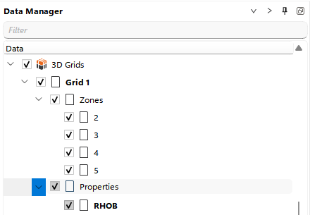
Every grid carries a Zones, a Properties and an Upscaled cells folder under its main folder in the Data Manager, listed even while they are still empty. You can access a context menu for managing these objects by right-clicking on them.

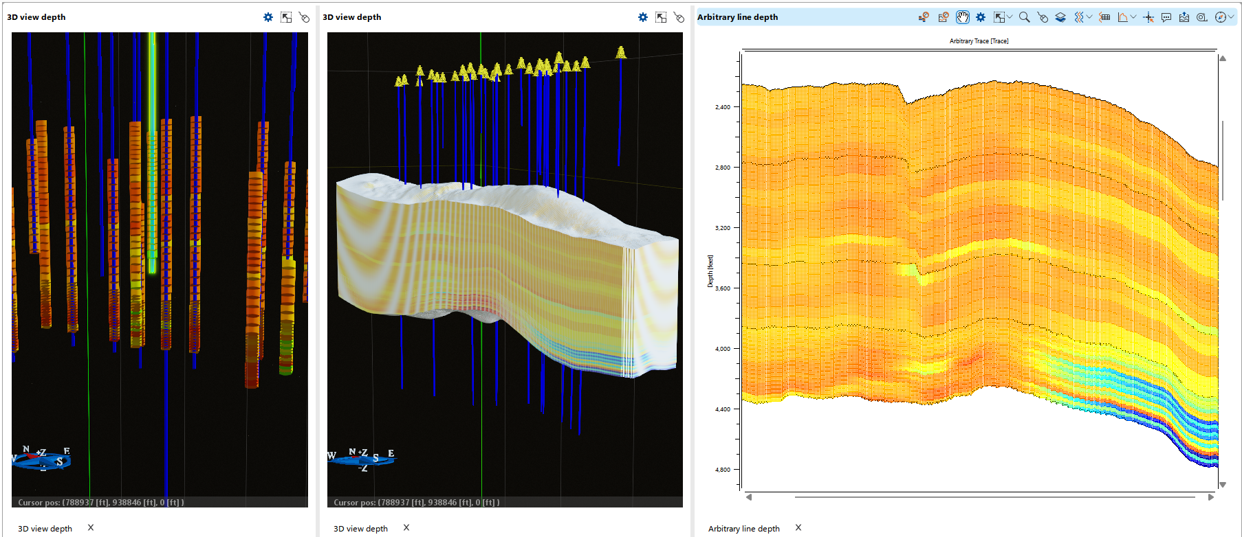
You can visualize the grid in 3D depth view as a complete cellular model, display grid cells along wells, and also view the grid in the section view for detailed analysis.

Visualization settings are available in the Visual Settings