The Edit LAS curve tool applies processing and editing operations to individual log curves.

This is useful for cleaning, correcting, or customizing log data before interpretation or correlation.

To open the wizard, go to the Petrophysics ribbon tab and, in the Logs group, click Edit LAS curve; on the button the caption is shortened to Edit curve.

You can also open the wizard for a particular curve from the Well correlation view: activate the Select interval tool on the view header toolbar and select the curve in its track. The wizard opens with that well and curve already chosen. To preset the interval as well, drag along the curve with the same tool: the wizard then enables Start and End on the MD range tab and fills them with the depths you covered. In a track that holds several curves, select the curve before you drag; otherwise the view reports Please, select a curve.

This route works only with the Select interval tool. While any other tool of the view header toolbar is active, clicking or dragging a curve leaves the wizard closed, so switch tools first or open the wizard from the Petrophysics ribbon tab.

The wizard consists of the following key areas:

1. Well and Curve Selection

At the top, select the target Well and the Curve (log) you wish to edit using the dropdown menus.

Enable Batch calculation to apply the same editing action to more than one well in a single run. The adjacent dropdown sets the scope of wells to process: besides All wells, it also lists the project's Filters, Folders and Well sections, so you can restrict the operation to a saved filter, a well folder or a well-section group. The Well and Curve dropdowns still choose which curve is edited in each well.

2. Depth Range

Select the depth range over which the operation will be applied. Options include:

• MD range: Measured Depth
• TVD range: True Vertical Depth
• TVDSS range: the vertical depth measured below mean sea level
• Markers range: Use tops/markers to define interval

On the MD range, TVD range, or TVDSS range tab, enable Start and/or End and enter the limiting depth values.

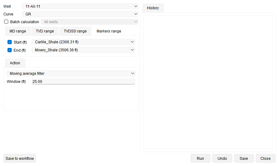
On the Markers range tab, enable Start and/or End and choose the corresponding marker. The example below applies Moving average filter between two selected markers.

3. Action – Log Editing Options

In this section, choose one of the available operations from the Action dropdown menu:

• Moving average filter: Smooths the log by averaging values within a specified window. Enter the window size in the current depth unit. The field is labelled Window (m) or Window (ft), depending on the measurement system.
• Median filter: Reduces noise by replacing each value with the median of its surrounding values within the defined window.
• Bandpass filter: Applies frequency-based filtering to isolate or remove specific ranges in the data.
• Depth shift: Shifts the entire curve vertically by a fixed amount. Useful for aligning logs when depth mismatches occur (e.g., from tool calibration errors).
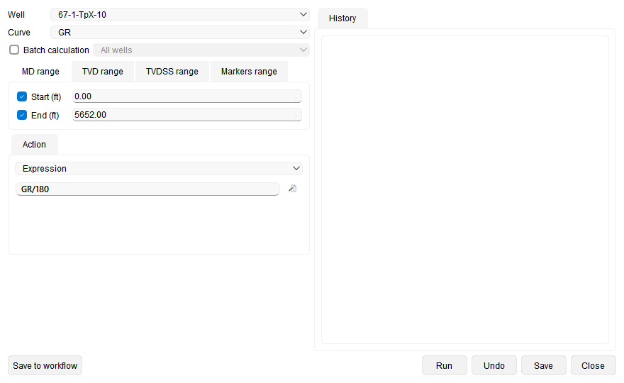
• Expression: Calculates new values for the selected curve from an expression. Enter the formula directly or click the calculator icon to build it from the available curves, operators and functions.
• Normalization: Rescales the curve with a linear transformation and writes the result to a new curve, so that equivalent logs from different wells or logging runs can be compared on a common response scale.
• Splice: Joins curves from LAS files on the same well on a common depth grid; see Splice LAS curves below.

The Expression action edits the selected curve in place. Enter only the expression, for example GR/180; do not add a name = prefix. If you include a prefix in the Log calculator opened from the calculator icon, g-Space asks you to remove it. You can reference the selected curve by its displayed name or by value. Curve names such as SP and SP1 are treated as separate identifiers.

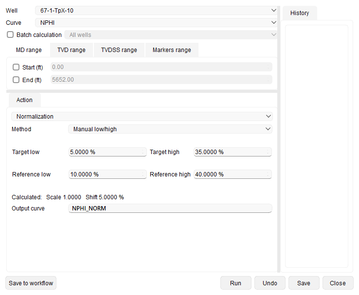
The Normalization action brings a curve onto a different response scale, for example to make equivalent logs from several wells or logging runs comparable before interpretation. Every method ends in the same linear transformation, Y = Scale × X + Shift, and they differ only in how the two coefficients are obtained. Select the method in the Method dropdown:

• Linear: Enter Scale and Shift yourself. Use this method when the normalization coefficients are already known.
• Manual low/high: Enter Target low, Target high, Reference low and Reference high in the units of the selected curve. g-Space derives the transformation that maps the two target values onto the two reference values.

Below the fields, Calculated: shows the Scale and Shift that the current settings produce. Output curve holds the name of the curve to create; it is pre-filled with the name of the selected curve and a _NORM suffix, and you can edit it.

Only the samples inside the selected depth or marker interval are transformed; the rest of the curve is copied unchanged. Null samples stay null and are never replaced by zeros, and the new curve keeps the units, description and curve type of the source curve.

For a normalization run, Save does not ask the general overwrite question: it writes the result under the name in Output curve, so the source curve is kept unless you set that name to the name of the source curve; if the editing session also contains edits of other curves, the usual prompt appears instead. With Batch calculation enabled, the same Scale and Shift are applied in every selected well, and wells whose curve has no valid samples in the selected interval are skipped and reported. Save to workflow stores the whole normalization setup, so the saved task reproduces the same result.

If the settings cannot produce a transformation, for example when Target high equals Target low, when Reference high equals Reference low, or when Output curve is empty, an explanatory message replaces the calculated coefficients, and Run and Save to workflow report the same message instead of running.

Splice LAS curves

Select a Well and a base Curve, then choose Splice in Action. Splice with lists eligible LAS files on that well in Start depth order. Files carrying the same curve mnemonic are included automatically; the base file is always included. Untick a partner file to leave it out, or use its Curve dropdown to choose a differently named curve. Run needs at least two included files.

Where included files overlap, Cut at starts at the overlap midpoint. Enter an MD value or bind the cut to a Marker; Mismatch at cut updates with the curve values and their difference. A gap or butt join has no cut, and gaps remain null in the result. When one file is contained within another, two cuts bound the patch, as shown below.

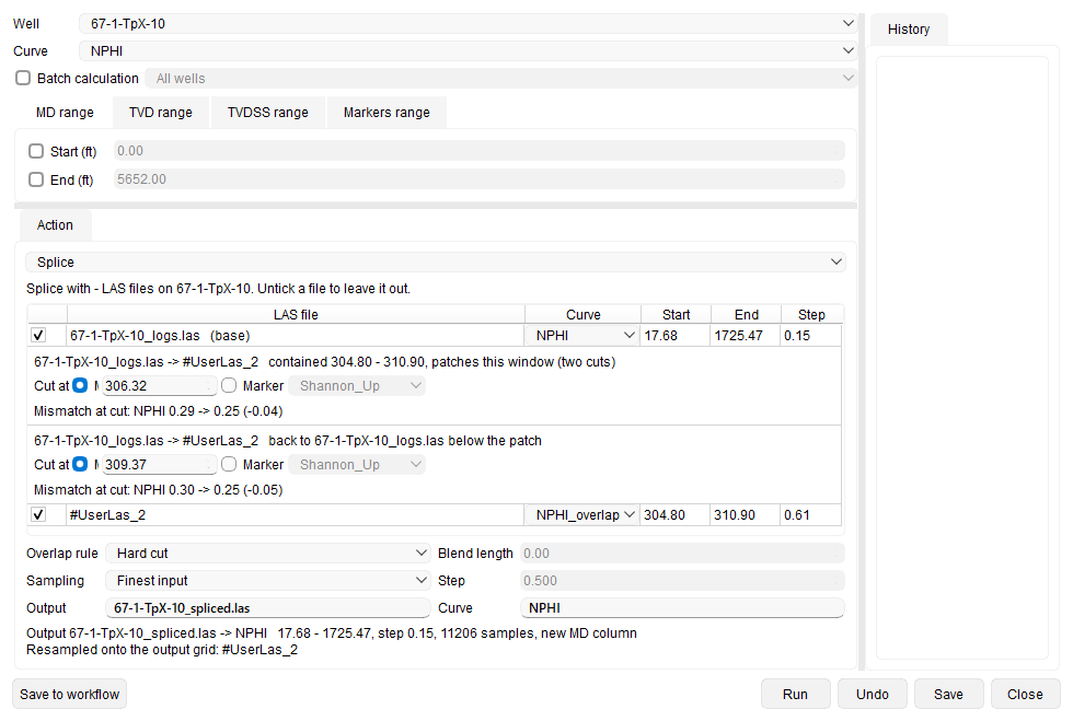
Overlap rule defaults to Hard cut, which switches sources at the cut. Blend zone linearly blends across the Blend length centered on the cut and limited to the overlap; a zero length leaves a hard cut. Fill nulls only keeps the base curve wherever it has a value and fills its null samples from the other included files. It has no cut rows.

Sampling defaults to Finest input, using the smallest included file step and resampling coarser files. Choose Custom and enter Step for a different output grid. The range tabs can limit the output extent for one well; without limits, it covers the union of the included file ranges. The summary reports the output extent, sample count, resampling and warnings. Null samples are not blended or interpolated across.

A partner curve with different units is refused by row. Different depth types or datums stop the splice until the conflicting file is unticked. Core curves and 2D array channels are excluded. Align mismatched depths with Depth shift before splicing.

Run adds one splice to History, and Undo removes the latest one. Save opens Save spliced curve and asks for LAS file name and Curve name, initially the well name followed by _spliced.las and the base mnemonic. The save dialog does not offer to overwrite the base curve. The output has its own MD column and is placed in the Spliced LAS set; input LAS files remain unchanged. The output curve retains source file and cut depth metadata.

To splice another curve on the same well, change Curve, choose partners as needed, and press Run again before saving. Another curve can be added to the named output LAS file only when its depth column matches. Otherwise, g-Space creates a uniquely named file and reports it. Saving the same curve name to a matching output file replaces that output curve.

With Batch calculation enabled, g-Space matches the selected mnemonic in each well's LAS files and recomputes midpoint cuts per well. A Marker bound cut uses that well's marker; a typed MD cut is not carried to other wells. Wells with fewer than two matching files are skipped and listed, and each completed well gets its own output file. The depth range tabs are ignored in batch mode. Save to workflow stores one Splice LAS curve job for the current setup.

4. History Panel

The History tab lists the actions run during the current editing session. Use Undo to remove the most recent action.

5. Buttons

• Save to workflow: Adds the configured edit as a workflow task.
• Run: Applies the selected action and adds it to History while keeping the wizard open. For actions other than Splice, the result is previewed in the Well correlation view: a red copy of the curve, named with an [Edited] prefix, appears in the same track or tracks as the original. Selecting this preview, or dragging along it with Select interval, keeps the wizard on the original curve; the preview disappears when you save the edits or close the wizard.
• Undo: Removes the most recently run action and restores the previous edit state.
• Save: Saves the accumulated edits and closes the wizard. When the general overwrite prompt appears, choose Yes to replace existing values, No to enter new curve names and keep the originals, or Cancel to return without saving. When you choose No and save new curve names, the new curves are added to the Data Manager and displayed immediately in the same Well correlation view track or tracks as their originals. They inherit the originals' display settings and use a contrasting color.
• Close: Closes the wizard. If the History contains unsaved actions, confirm whether to discard them.

Deleting a single curve

To delete one log curve without affecting the rest of the LAS, right-click that curve in the Data Manager (in the well's log list or under All curves) and choose Remove. g-Space asks for confirmation (Do you want to remove selected las curves?) and then removes only the selected curve, leaving the other curves in the file unchanged.