The Trace Header Crossplotting feature in g-Viewer allows users to visualize relationships between trace headers by plotting two headers on the X and Y axes and using a third header for color-coding. This provides a powerful tool for data quality control (QC), trend analysis, and anomaly detection in seismic datasets.
Selecting Trace Headers
•Open the Trace Headers Table and identify the headers you want to plot.
•Right-click on a trace header column and choose "Show as Horizontal Axis" to assign it to the X-axis.
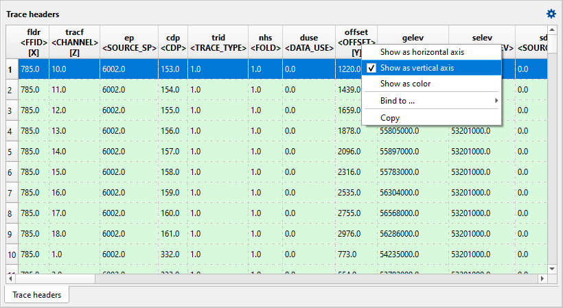
•Similarly, right-click another trace header column and select "Show as Vertical Axis" for the Y-axis.
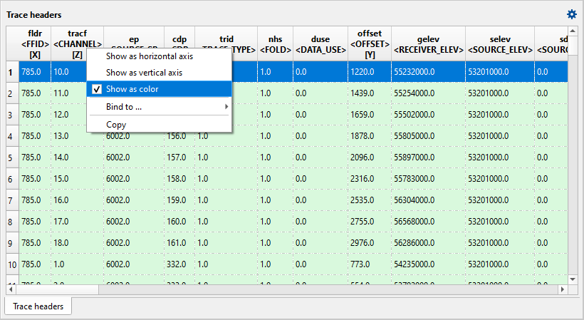
•Finally, assign a third trace header to be displayed as color variation in the plot.
The resultant plot can be seen in the QC graph view.
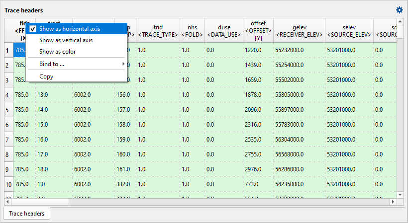
Here we are selecting FFID as horizontal axis. To do that, user should right click on the FFID column and choose Show as horizontal axis option. Similarly we ca select the other trace headers for vertical axis (In this case OFFSET) and color to display.
Finally we can select CHANNEL column as a color for the QC graph display.
The resultant QC graph is as shown below.
![]()
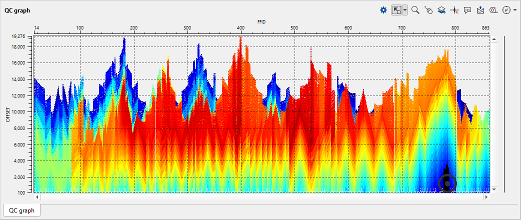
Likewise the user can cross plot any of 3 trace headers to quickly visualize and QC the trace headers in a more efficient way.
When is This Tool Useful?
1. Quality Control of Trace Headers
•Detecting inconsistent header values, such as unexpected offsets or incorrect shot numbers.
•Identifying missing or duplicate traces in the dataset.
2. Checking Source-Receiver Geometry
•Verifying the distribution of offsets in relation to FFID to ensure a uniform shot spacing.
•Identifying irregular shot patterns that may indicate acquisition errors.
3. Validating Marine and Land Seismic Acquisition Data
•In marine surveys, analyzing the correlation between shot point number, receiver distance, and channel number to detect potential positioning errors.
•In land seismic surveys, visualizing the relationship between source-receiver azimuths, offsets, and elevation to check terrain effects.
4. Identifying Instrumentation or Processing Errors
•Checking variations in trace scaling, gains, or filter application by plotting trace gain vs. channel number.
•Detecting systematic errors in seismic sensors or processing workflows.
5. Detecting Geometry and Navigation Errors
•Crossplotting CDP (Common Depth Point) vs. Offset and color-coding by Shot Point to detect incorrect CDP binning.
•Identifying overlapping or missing CDP bins in land and marine seismic acquisition.
•Checking for navigation inconsistencies by plotting Source X vs. Source Y and color-coding by FFID.