Module name Spherical divergence correction
Spherical divergence correction is applied prior to prestack data to compensate the energy loss (amplitude decay) during the wave propagation. As the wavefront expands the energy is spread over a wider area and the amplitude decays with distance from the source. This amplitude decay is called spherical divergence.
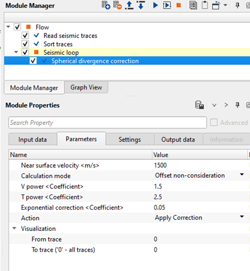
To compensate the amplitude decay, we need to test different combinations of spherical divergence corrections viz., T 2, T 2V and T 2V 2 with a single velocity function which is typically "Near surface velocity".
If you choose the offset dependent then the equation will be
• SCALAR (t) = (T * V2/ V0) * SQRT (1 + A) , where
• A = (V2– V02) * X2/ (T02* V4), and
• X = offset of this trace,
• T = trace time at offset X,
• T 0= zero-offset time of this event,
• V = stacking velocity, extracted at time T0,
• V 0= surface velocity (extracted from velocity function at time 0), and we assume that T and T0 are related by the NMO equation:
• T2= T02+ (X/V)2
If we choose the offset independent then the equation will be
A = A0(t)+1/
Where A - corrected amplitude at time t
A0 - Observed amplitude at time t
t - two way travel time
In this workflow, we are reading the geometry assigned gathers by using "Read seismic traces" and sorting the data by FFID and Channel as Grouping and Sorting respectively. Inside the seismic loop, we are adding Spherical divergence correction module.
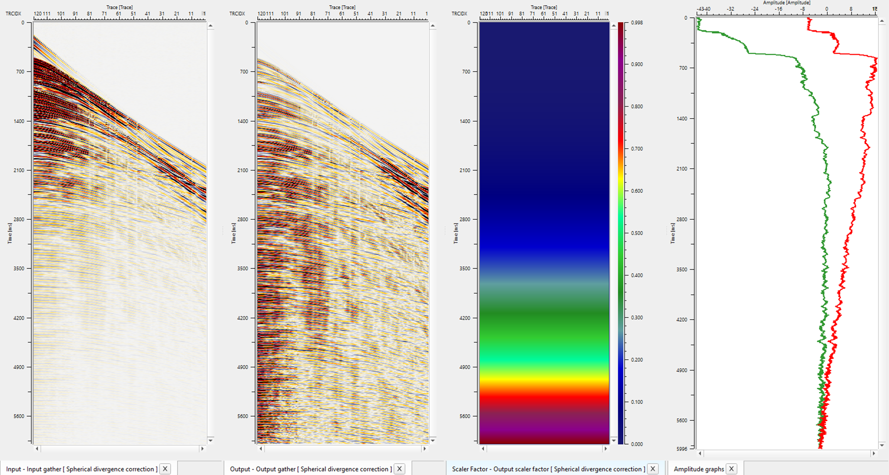
As per the data requirements, test the appropriate parameters. We'll get 4 QC displays for Spherical divergence as shown below. It'll be Input gather, Output gather after spherical divergence correction, Scale factor and Amplitude Graph.