The Base properties module provides a set of fundamental calculations commonly used in petrophysical and geomechanical analysis.
Each tab represents an individual calculator that generates a new log curve for the selected well or a batch of wells.
The module allows users to specify input parameters, define a calculation interval, and visualize the resulting curve before saving it to the project.
Hydrostatic Pressure
Calculates the hydrostatic pressure as a function of depth using the selected fluid density.
The relationship is defined by:
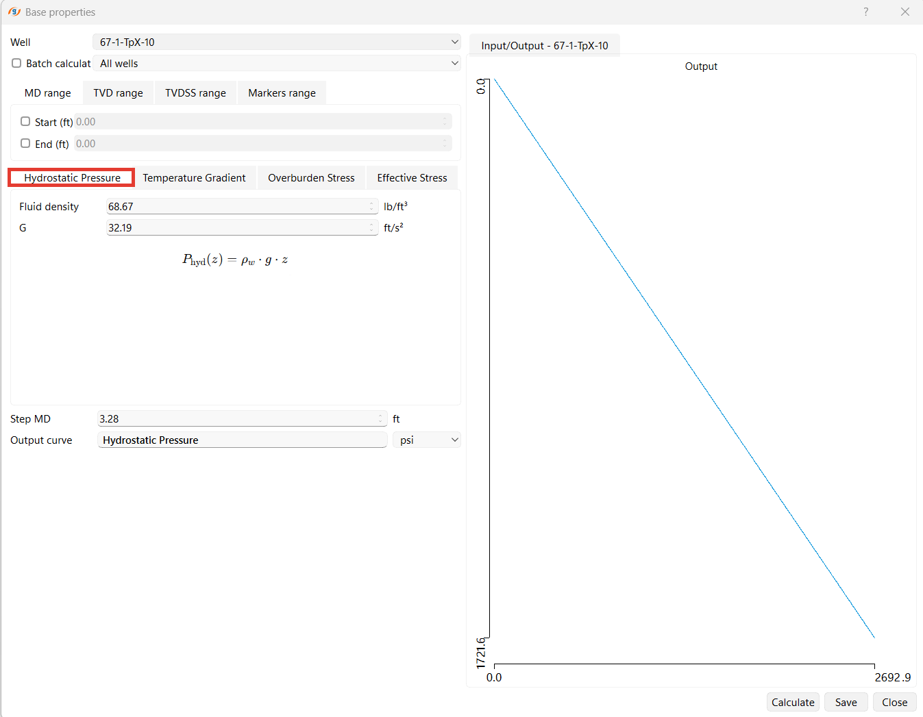
where
•ρw – fluid density,
•g – gravitational acceleration,
•z – depth.
Input parameters:
•Fluid density (kg/m³ or lb/ft³)
•Gravity constant (m/s² or ft/s²)
•Measured depth range and step
Output: Hydrostatic pressure curve (MPa or psi)
Temperature Gradient
Computes the temperature distribution with depth using a constant surface temperature and geothermal gradient.
The formula applied:
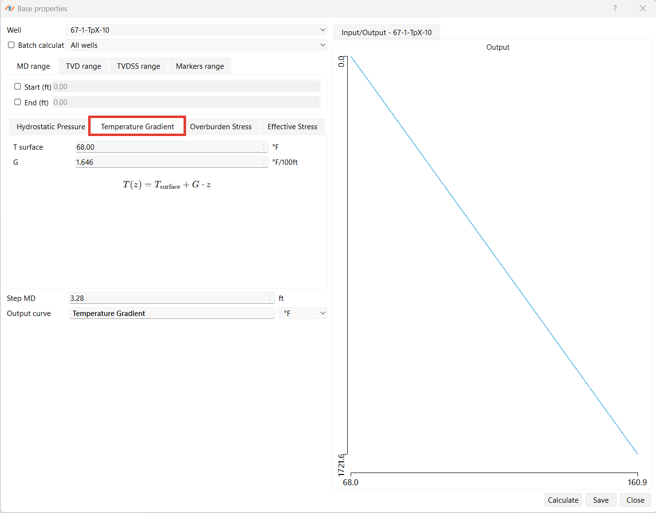
where
•Tsurface – surface temperature,
•G – geothermal gradient,
•z – depth.
Input parameters:
•Surface temperature (°C or °F)
•Temperature gradient (°C/100 m or °F/100 ft)
•Depth step
Output: Temperature Gradient curve
Overburden Stress
Estimates the vertical stress resulting from the weight of the overlying sediments.
The calculation integrates the rock bulk density curve over depth:
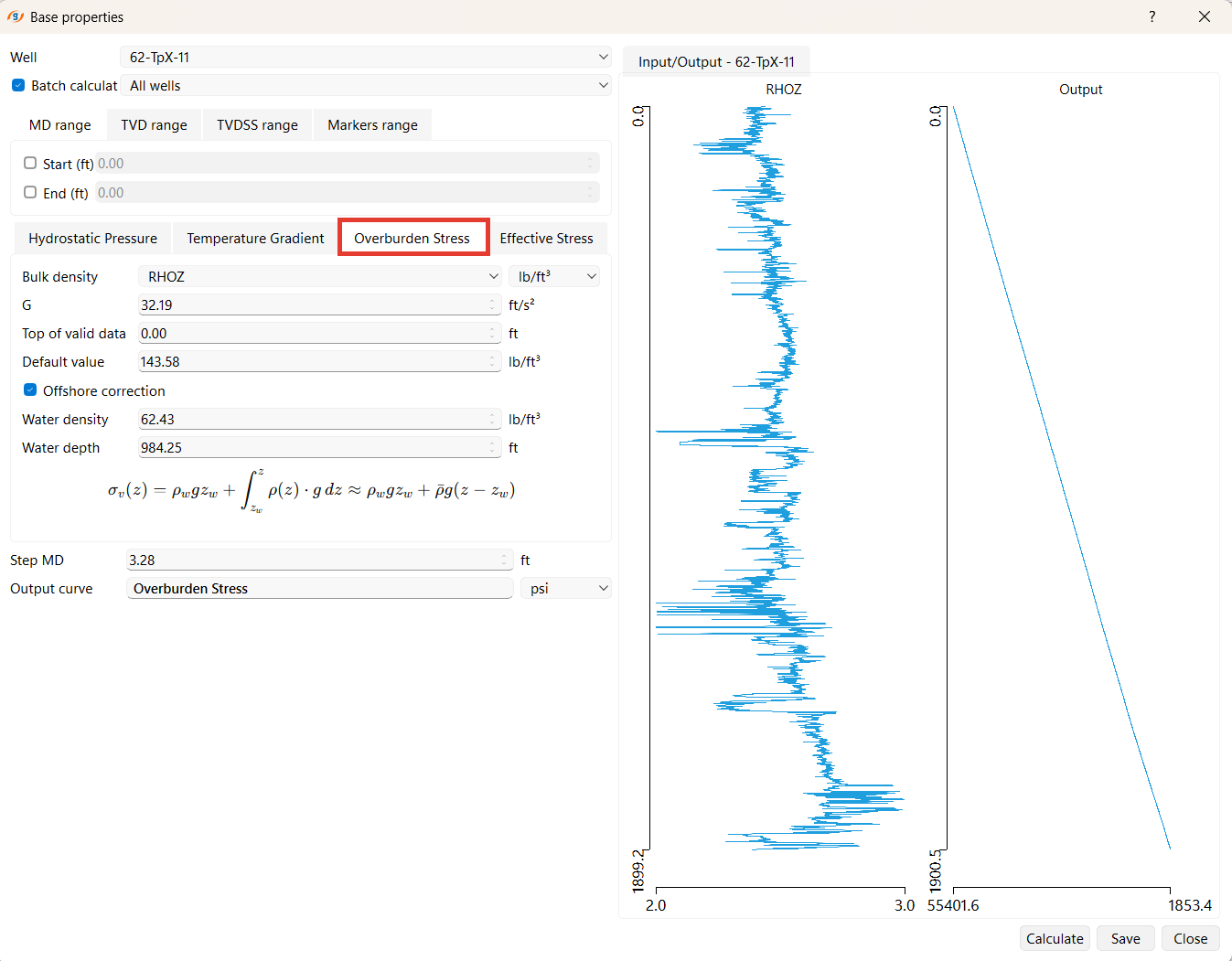
where
•ρ – bulk density,
•g – gravitational acceleration.
Input parameters:
•Bulk density log
•Gravity constant
•Depth interval and step
Output: Overburden stress curve (MPa or psi)
Effective Stress
Determines the effective stress by subtracting pore pressure from total overburden stress:
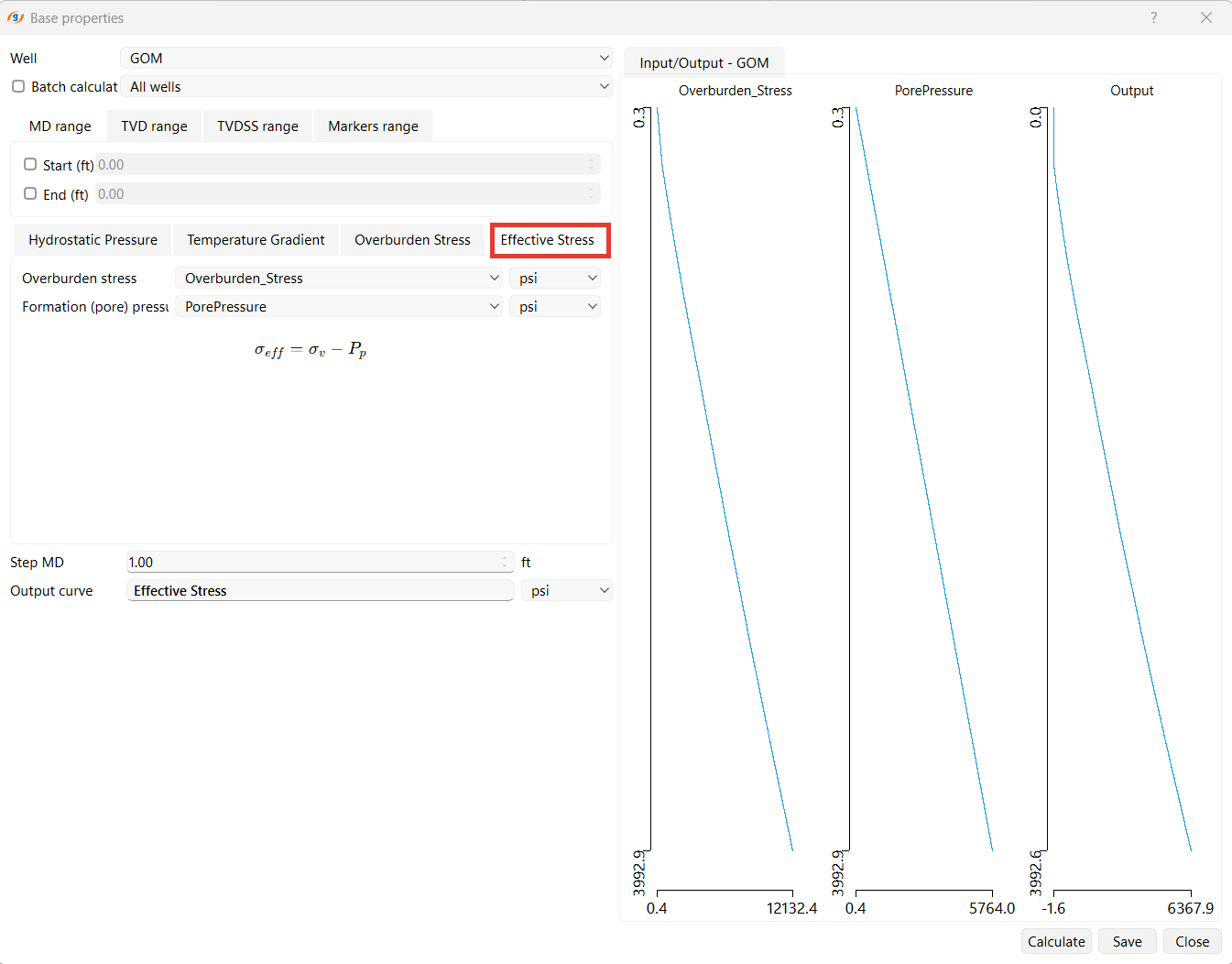
where
•σv – overburden stress,
•Pp – pore pressure.
Input parameters:
•Overburden stress curve
•Pore pressure curve
Output: Effective stress curve (MPa or psi)